Tag Archives: exponential smoothing

Video Friday – Volatility

Here are a couple of short YouTube videos from Bionic Turtle on estimating a GARCH (generalized autoregressive conditional heteroskedasticity) model and the simpler exponentially weighted moving average (EWMA) model.

GARCH models are designed to capture the clustering of volatility illustrated in the preceding post.

Forecast volatility with GARCH(1,1)

The point is that the parameters of a GARCH model are estimated over historic data, so the model can be utilized prospectively, to forecast future volatility, usually in the near term.

EWMA models, insofar as they put more weight on recent values, than on values more distant back in time, also tend to capture clustering phenomena.

Here is a comparison.

EWMA versus GARCH(1,1) volatility

Several of the Bionic Turtle series on estimating financial metrics are worth checking out.

Seasonal Sales Patterns – Stylized Facts

Seasonal sales patterns in the United States are more or less synchronized with Europe, Japan, China, and, to a lesser extent, the rest of the world.

Here are some stylized facts:

  1. Sales tend to peak at the end of the calendar year. This is the well-known “Christmas effect,” and is a strong enough factor to “cannibalize” demand, to an extent, at the first of the following year.
  2. Sales of final goods tend to be lower – in terms of growth rates and, in some cases, absolutely, in the first calendar quarter of the year.
  3. Supply chain effects, related to pulses of sales of final goods, can be identified for various lines of production depending on production lead times. Semiconductor orders, for example, tend to peak earlier than sales of consumer electronics, which are sharply influenced by the Christmas season.

To validate this picture, let me offer some evidence.

First, consider retail and food service sales data for the US, a benchmark of consumer activity – the recently discussed data downloaded from FRED.

Applying the automatic model selection of the Hyndman R Forecast package, we get a decomposition of this time series into level, trend, and seasonals, as shown in the following diagram.

Rplotrs

The optimal exponential smoothing forecast model is a model with a damped trend and multiplicative seasonals.

If we look at the lower part of this diagram, we see that the seasonal factor for December – which is shown by the major peaks in the curve – is a multiple of more than 1.15. On the other hand, the immediately following month – January – shows a multiple of 0.9. These factors are multiplied into the product of the level and trend to get the sales for December and January. In other words, you can suppose that, roughly speaking, December retail sales will be 15 percent above trend, while January sales will be 90 percent of trend.

And, if you inspect this diagram in the lower panel carefully, you can detect the lull in late summer and fall in retail sales.

With “just-in-time” inventories and lean production models, actual production activity closely tracks these patterns in final demand – although it does take some lead time to produce stuff.

These stylized facts have not changed in their outlines since the ground-breaking research of Jeffrey Miron in the the late 1980’s. Miron refers to a worldwide seasonal cycle in aggregate economic activity whose major features are a fourth quarter boom in output.., a third quarter trough in manufacturing production, and a first quarter trough in all economic activity.

The Effects of Different Calendars – the Chinese New Year and Ramadan

The Gregorian calendar has achieved worldwide authority, and almost every country follows on the conventions of counting the year (currently 2014).

The Chinese calendar, however, is still important for determining the timing of festivals for Chinese communities around the world, and, especially, in China.

GRAPHICS TEMPLATE 2006

Similarly, the Islamic calendar governs the timing of important ritual periods and religious festivals – such as the month of Ramadan, which falls in June and July in 2014.

Because these festival periods overlap with multiple Gregorian months, there can be significant localized impacts on estimates of seasonal variation of economic activity.

Taiwanese researchers looking at this issue find significant holiday effects, related the fact that,

The three most important Chinese holidays, Chinese New Year, the Dragon-boat Festival, and Mid-Autumn Holiday have dates determined by a lunar calendar and move between two solar months. Consumption, production, and other economic behavior in countries with large Chinese population including Taiwan are strongly affected by these holidays. For example, production accelerates before lunar new year, almost completely stops during the holidays and gradually rises to an average level after the holidays.

Similarly, researchers in Pakistan consider the impacts of the Islamic festivals on standard macroeconomic and financial time series.

Wrap on Exponential Smoothing

Here are some notes on essential features of exponential smoothing.

  1. Name. Exponential smoothing (ES) algorithms create exponentially weighted sums of past values to produce the next (and subsequent period) forecasts. So, in simple exponential smoothing, the recursion formula is Lt=αXt+(1-α)Lt-1 where α is the smoothing constant constrained to be within the interval [0,1], Xt is the value of the time series to be forecast in period t, and Lt is the (unobserved) level of the series at period t. Substituting the similar expression for Lt-1 we get Lt=αXt+(1-α) (αXt-1+(1-α)Lt-2)= αXt+α(1-α)Xt-1+(1-α)2Lt-2, and so forth back to L1. This means that more recent values of the time series X are weighted more heavily than values at more distant times in the past. Incidentally, the initial level L1 is not strongly determined, but is established by one ad hoc means or another – often by keying off of the initial values of the X series in some manner or another. In state space formulations, the initial values of the level, trend, and seasonal effects can be included in the list of parameters to be established by maximum likelihood estimation.
  2. Types of Exponential Smoothing Models. ES pivots on a decomposition of time series into level, trend, and seasonal effects. Altogether, there are fifteen ES methods. Each model incorporates a level with the differences coming as to whether the trend and seasonal components or effects exist and whether they are additive or multiplicative; also whether they are damped. In addition to simple exponential smoothing, Holt or two parameter exponential smoothing is another commonly applied model. There are two recursion equations, one for the level Lt and another for the trend Tt, as in the additive formulation, Lt=αXt+(1-α)(Lt-1+Tt-1) and Tt=β(Lt– Lt-1)+(1-β)Tt-1 Here, there are now two smoothing parameters, α and β, each constrained to be in the closed interval [0,1]. Winters or three parameter exponential smoothing, which incorporates seasonal effects, is another popular ES model.
  3. Estimation of the Smoothing Parameters. The original method of estimating the smoothing parameters was to guess their values, following guidelines like “if the smoothing parameter is near 1, past values will be discounted further” and so forth. Thus, if the time series to be forecast was very erratic or variable, a value of the smoothing parameter which was closer to zero might be selected, to achieve a longer period average. The next step is to set up a sum of the squared differences of the within sample predictions and minimize these. Note that the predicted value of Xt+1 in the Holt or two parameter additive case is Lt+Tt, so this involves minimizing the expression Sqerroreq Currently, the most advanced method of estimating the value of the smoothing parameters is to express the model equations in state space form and utilize maximum likelihood estimation. It’s interesting, in this regard, that the error correction version of ES recursion equations are a bridge to this approach, since the error correction formulation is found at the very beginnings of the technique. Advantages of using the state space formulation and maximum likelihood estimation include (a) the ability to estimate confidence intervals for point forecasts, and (b) the capability of extending ES methods to nonlinear models.
  4. Comparison with Box-Jenkins or ARIMA models. ES began as a purely applied method developed for the US Navy, and for a long time was considered an ad hoc procedure. It produced forecasts, but no confidence intervals. In fact, statistical considerations did not enter into the estimation of the smoothing parameters at all, it seemed. That perspective has now changed, and the question is not whether ES has statistical foundations – state space models seem to have solved that. Instead, the tricky issue is to delineate the overlap and differences between ES and ARIMA models. For example, Gardner makes the statement that all linear exponential smoothing methods have equivalent ARIMA models. Hyndman points out that the state space formulation of ES models opens the way for expressing nonlinear time series – a step that goes beyond what is possible in ARIMA modeling.
  5. The Importance of Random Walks. The random walk is a forecasting benchmark. In an early paper, Muth showed that a simple exponential smoothing model provided optimal forecasts for a random walk. The optimal forecast for a simple random walk is the current period value. Things get more complicated when there is an error associated with the latent variable (the level). In that case, the smoothing parameter determines how much of the recent past is allowed to affect the forecast for the next period value.
  6. Random Walks With Drift. A random walk with drift, for which a two parameter ES model can be optimal, is an important form insofar as many business and economic time series appear to be random walks with drift. Thus, first differencing removes the trend, leaving ideally white noise. A huge amount of ink has been spilled in econometric investigations of “unit roots” – essentially exploring whether random walks and random walks with drift are pretty much the whole story when it comes to major economic and business time series.
  7. Advantages of ES. ES is relatively robust, compared with ARIMA models, which are sensitive to mis-specification. Another advantage of ES is that ES forecasts can be up and running with only a few historic observations. This comment applied to estimation of the level and possibly trend, but does not apply in the same degree to the seasonal effects, which usually require more data to establish. There are a number of references which establish the competitive advantage in terms of the accuracy of ES forecasts in a variety of contexts.
  8. Advanced Applications.The most advanced application of ES I have seen is the research paper by Hyndman et al relating to bagging exponential smoothing forecasts.

The bottom line is that anybody interested in and representing competency in business forecasting should spend some time studying the various types of exponential smoothing and the various means to arrive at estimates of their parameters.

For some reason, exponential smoothing reaches deep into actual process in data generation and consistently produces valuable insights into outcomes.

Exponential Smoothing – Black Box Examples

The reason why most people would be interested in and concerned with exponential smoothing (ES) is that it is an effective forecasting technique.

So, with that in mind, I want to discuss two automatic forecasting programs – Forecast Pro and Hyndman’s Forecast program for R – applied to a monthly time series for public construction spending in the US. I do this more or less “black box” in that I am not spending a lot of time on the underlying theory – which is basically a state space model framework – but focus on the process of getting the forecasts and their comparison.

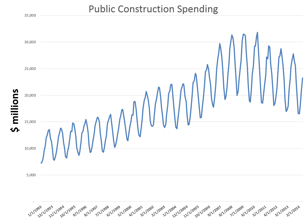
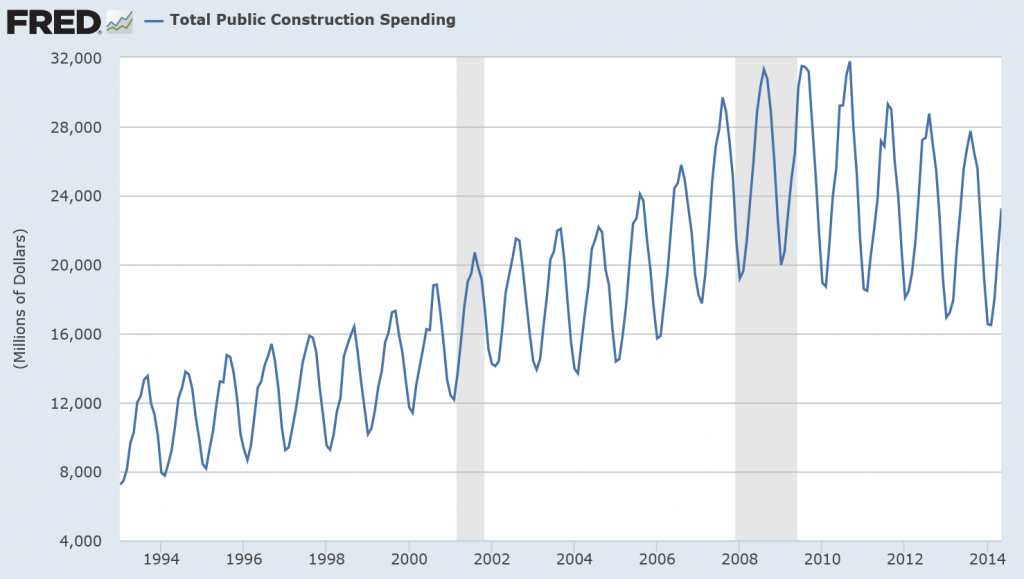
I am testing these programs with a backcasting exercise. Thus, the data for this time series, available from FRED begin January 1993 and extend through May 2014. However, I only use data up to May 2010 to develop forecasting models with these programs. Then, I can compare the forecasts from the models with actual values. So instead of forecasting, you might say I am backcasting. Sometimes this is also called retrodiction, in contrast to prediction.

FREDCS

My plan is to feed both programs data up to and including May 2010, in order to forecast values for the next 24 months.

Forecast Pro

Data input is the first step, and this can be accomplished with Forecast Pro by means of an Excel spreadsheet. There are requirements for how you lay out the data. Basically, the first column, below the first six rows, can contain dates. The first time series is placed in the second column, after noting its name and description, the starting year, starting period (month, quarter, etc), periods per year, and any information on cycles. Then, of course, you store the spreadsheet in a directory where the program can pick it up – but all that is covered in the Forecast Pro manual.

Here’s what the program panel looks like, after you trigger the automatic forecasting procedure (click to enlarge).

FPro

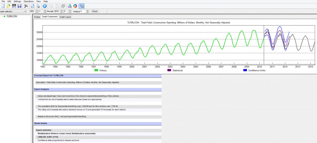
So basically you see a graph of the historic data you are feeding into the program. If you look down to Model Details you will see that expert selection picked a multiplicative Winters linear trend, multiplicative seasonality model. The estimated parameters are then given.

Above this, under Expert Analysis, the screen tells you that it looked at both Box-Jenkins (ARIMA) and ES models, picking the ES model based on out-of-sample tests.

Further down on this screen (not shown), the program lists the forecasts, which are graphed with confidence intervals above (shown).

I’ll discuss these forecasts, but first let me say a few words about the Hyndman R Forecast package analysis.

The Hyndman R Forecast Package

R is very big in some of the enterprise IT outfits. I have friends, for example, who view it as essential, and who have helped me recently come up to speed, to an extent, in using it.

After some fumbling around, I settled on running my R programs in R Studio. There is something called the Comprehensive R Archive Network (CRAN) with important open source R programs. Hyndman et al have their Forecast program listed there, and it pops up in R Studio, which is hugely convenient.

Again, there is an issue of data input. In this case, correctly positioning a csv spreadsheet file works well.

The R code I used to generate ES forecasts is as follows:

R

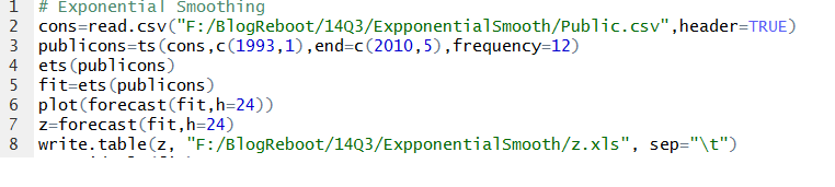
Note I screw up the spelling of ExponentialSmooth in naming the subdirectory. Oh well.

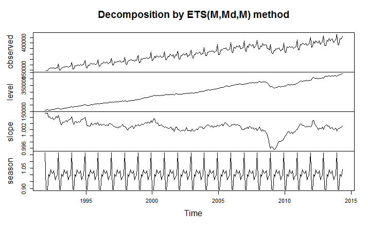
So after you import the csv file with the read command, you convert it to a time series format. Then, you can apply the operation ets(.) to the time series file, producing the parameters of the optimal ES model, based on comparisons of Akaike information criteria from the maximum likelihood estimations used to calculate the parameters of all the models.

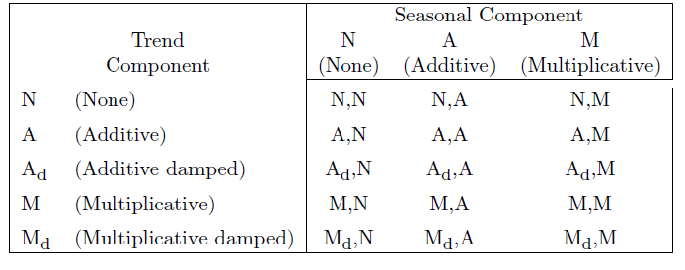
Forecast selects ETS(M,Ad,M) as the optimal model. This indicates an additive trend is used, but is damped, and that the seasonal effects are multiplicative – more or less as in the Forecast Pro analysis.

The Forecasts

I called for 24 months of forecasts from both programs.

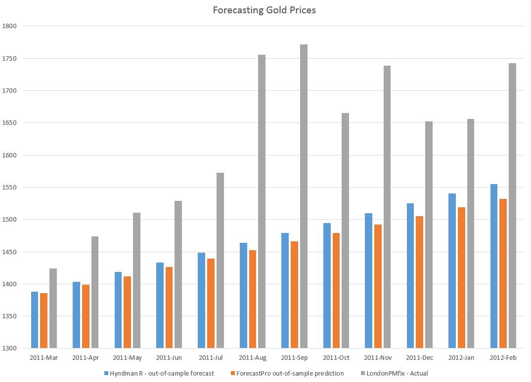
Here is a table comparing the forecasts from both packages with the actual values of this public construction time series.

TableFPH

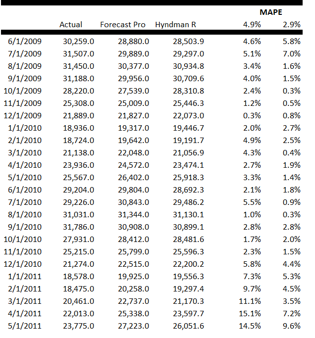
The Hyndman et al R Forecast package produces significantly lower Mean Absolute Percentage Error (MAPE) than Forecast Pro in these forecasts – 2.9% compared with 4.9%.

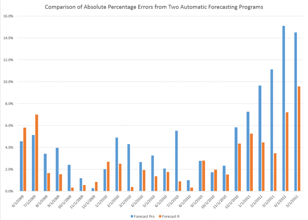
Here is a chart comparing the absolute percent error by month over the forecast horizon.

compRFP

Conclusions

This particular example is a case of random selection. I really have not run other forecasts with this data and these two models, except for actual future projections. So it’s interesting that an explicitly damped linear trend applied to these data generates a superior forecast to whatever it is that Forecast Pro does.

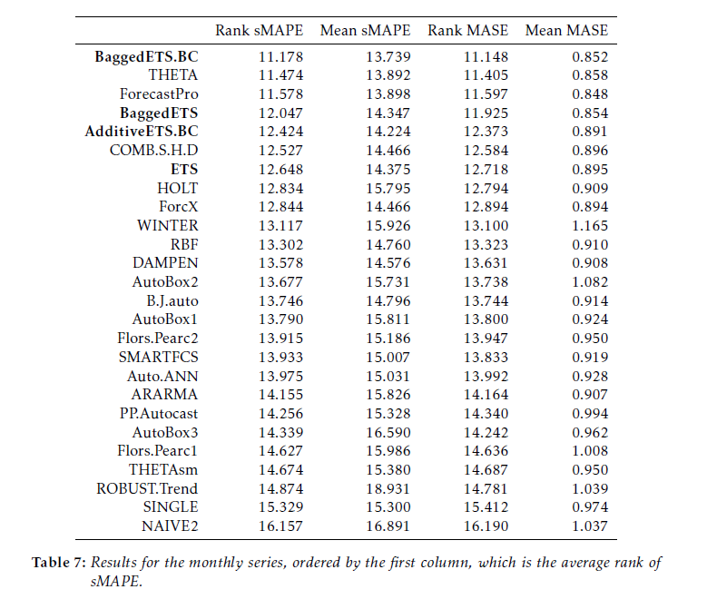
But readers should be aware that, in many instances, Forecast Pro can slightly outperform the R Forecast program, as Hyndman and coauthors document in a critical paper on this automatic forecasting setup in R.

However, the performance of the two programs is very similar.

In general, I would suggest that non-mathematical users, or folks not used to developing computer programs, stick with Forecast Pro, probably getting the company or organization you work for to pony up several hundred to several thousand dollars to get what you need for the scale of the forecasting problem at hand. Incidentally, I should be getting commissions for boosting this program, as often as I do, but I have no connection with the company.

For more mathematically sophisticated users, I strongly recommend getting up to speed on the R Forecast package and other R packages.

Both would be nice to use together. The R programs can support an interesting research effort, doing all sorts of clever things like fitting splines to the data, boosting, and bagging. Forecast Pro on the other hand is great if you have to produce a large number of forecasts and do not have time to dwell too much on the details of each series.

Exponential Smoothing – I

As I wrote recently, most business forecasting assignments are relatively simple. You collect the data (often the most challenging part), and plug this data into an automatic forecasting program. The program probably applies some type of exponential smoothing (ES) to produce forecasts for a horizon of a few periods ahead, and, bam, there you have it. The rest is presentation, developing the “story” and so forth.

So what about this exponential smoothing? What’s basically involved? What are the differences between exponential smoothing and the other primary univariate forecasting technique – ARIMA or Box-Jenkins modeling? What are these automatic forecasting programs, and which ones are best?

All good questions, and, if you are interested or involved in forecasting, the answers are good to rehearse from time to time.

Level, Trend, Seasonality – Components of Time Series

Exponential smoothing originated with the work of Brown and Holt for the US Navy (see the discussion in Gardiner). The perspective was not theoretical, but applied.

Nevertheless, there is an intuitive aspect to exponential smoothing (ES). That has to do with the decomposition of time series into components – such as level, trend, and seasonal effects.

So, applying the algorithms of ES to some time series Xt t=1,2,…,n, we extract estimates of the level Lt, trend Tt, and seasonal component, St, so that at any time t, we can express Xt as

Xt = Lt + Tt + St

This would be an additive model.

It’s also possible that the time series Xt could be multiplicative, as in

Xt = LtTtSt

By way of example, consider the following time series for public construction spending in the US, obtained from FRED (Federal Reserve Economic Data).

PCS

Now if you look closely, it’s clear there are strongly delineated seasonal effects. Furthermore, these seasonal variations appear to fluctuate more or less in proportion to the annual levels of the series. Thus, the variation is considerably more over a year, when spending is at a $25 billion level, than it does at a $10 billion level.

And the fact that these levels are different, and the series does not simply oscillate around a single level, indicates that there is probably a meaningful trend component to this time series.

Automatic Forecasting Programs

These are the considerations that you take into account in building an exponential smoothing model.

Now it is possible to create ES models within the framework of a spreadsheet. Thus, ES models have smoothing parameters which can be set by minimizing a squared sum of forecast errors over historic data. In Microsoft’s Excel, you can use Solver to do this, once you set up the recursion equations for level, trend, and seasonal components or effects.

In coming posts, I want to show how this can be done for a simple example.

But really, setting up spreadsheets to estimate exponential smoothing models can be laborious, since you need a separate set of computations for every possible model. In addition to the additive and purely multiplicative models shown above, for example, there can be hybrid cases – multiplicative seasonality but additive trend, and so forth.

So it’s a good idea to equip yourself with one of the several, good automatic forecasting programs out there to speed model identification and evaluation.

I will have reference to two such automatic forecasting programs in coming posts – Forecast Pro and Rob Hyndman’s Forecast package in R. I’ll make comparisons between these programs. A demo version of Forecast Pro is available for download for free, but it is a commercial package with various options at various price steps. Hyndman’s R forecasting package, on the other hand, is open source software and free, as is the R platform. While this sounds like an unbeatable advantage, there always are questions of bugs and performance – which in this case seem to be to be resolved for reasons we can discuss.

What’s The Big Deal?

Finally, the reason why ES forecasting is so widely applied is that, in many cases, it produces forecasts which are of comparable or superior accuracy to other univariate forecasting approaches.

ES has performed well, for example, in international forecasting competitions, including the widely-publicized M-competitions.

There also is a link between exponential smoothing and the Kalman filter. So ES is in a sense an adaptive forecasting approach. For example, ES weights more recent observations more heavily than observations more distant in the past, unlike a regression trend model.

Finally, recent research has provided statistical pedigree to exponential smoothing, rescuing it in a sense from consignment to “a purely ad hoc” approach. Thus, there is a direct link between time series that embody a random walk or random walk with drift and exponential smoothing.

Automatic Forecasting Programs – the Hyndman Forecast Package for R

I finally started learning R.

It’s a vector and matrix-based statistical programming language, a lot like MathWorks Matlab and GAUSS. The great thing is that it is free. I have friends and colleagues who swear by it, so it was on my to-do list.

The more immediate motivation, however, was my interest in Rob Hyndman’s automatic time series forecast package for R, described rather elegantly in an article in the Journal of Statistical Software.

This is worth looking over, even if you don’t have immediate access to R.

Hyndman and Exponential Smoothing

Hyndman, along with several others, put the final touches on a classification of exponential smoothing models, based on the state space approach. This facilitates establishing confidence intervals for exponential smoothing forecasts, for one thing, and provides further insight into the modeling options.

There are, for example, 15 widely acknowledged exponential smoothing methods, based on whether trend and seasonal components, if present, are additive or multiplicative, and also whether any trend is damped.

15expmethods

When either additive or multiplicative error processes are added to these models in a state space framewoprk, the number of modeling possibilities rises from 15 to 30.

One thing the Hyndman R Package does is run all the relevant models from this superset on any time series provided by the user, picking a recommended model for use in forecasting with the Aikaike information criterion.

Hyndman and Khandakar comment,

Forecast accuracy measures such as mean squared error (MSE) can be used for selecting a model for a given set of data, provided the errors are computed from data in a hold-out set and not from the same data as were used for model estimation. However, there are often too few out-of-sample errors to draw reliable conclusions. Consequently, a penalized method based on the in-sample  t is usually better.One such approach uses a penalized likelihood such as Akaike’s Information Criterion… We select the model that minimizes the AIC amongst all of the models that are appropriate for the data.

Interestingly,

The AIC also provides a method for selecting between the additive and multiplicative error models. The point forecasts from the two models are identical so that standard forecast accuracy measures such as the MSE or mean absolute percentage error (MAPE) are unable to select between the error types. The AIC is able to select between the error types because it is based on likelihood rather than one-step forecasts.

So the automatic forecasting algorithm, involves the following steps:

1. For each series, apply all models that are appropriate, optimizing the parameters (both smoothing parameters and the initial state variable) of the model in each case.

2. Select the best of the models according to the AIC.

3. Produce point forecasts using the best model (with optimized parameters) for as many steps ahead as required.

4. Obtain prediction intervals for the best model either using the analytical results of Hyndman et al. (2005b), or by simulating future sample paths..

This package also includes an automatic forecast module for ARIMA time series modeling.

One thing I like about Hyndman’s approach is his disclosure of methods. This, of course, is in contrast with leading competitors in the automatic forecasting market space –notably Forecast Pro and Autobox.

Certainly, go to Rob J Hyndman’s blog and website to look over the talk (with slides) Automatic time series forecasting. Hyndman’s blog, mentioned previously in the post on bagging time series, is a must-read for statisticians and data analysts.

Quick Implementation of the Hyndman R Package and a Test

But what about using this package?

Well, first you have to install R on your computer. This is pretty straight-forward, with the latest versions of the program available at the CRAN site. I downloaded it to a machine using Windows 8 as the OS. I downloaded both the 32 and 64-bit versions, just to cover my bases.

Then, it turns out that, when you launch R, a simple menu comes up with seven options, and a set of icons underneath. Below that there is the work area.

Go to the “Packages” menu option. Scroll down until you come on “forecast” and load that.

That’s the Hyndman Forecast Package for R.

So now you are ready to go, but, of course, you need to learn a little bit of R.

You can learn a lot by implementing code from the documentation for the Hyndman R package. The version corresponding to the R file that can currently be downloaded is at

http://cran.r-project.org/web/packages/forecast/forecast.pdf

Here are some general tutorials:

http://cran.r-project.org/doc/contrib/Verzani-SimpleR.pdf

http://cyclismo.org/tutorial/R/

http://cran.r-project.org/doc/manuals/R-intro.html#Simple-manipulations-numbers-and-vectors

http://www.statmethods.net/

And here is a discussion of how to import data into R and then convert it to a time series – which you will need to do for the Hyndman package.

I used the exponential smoothing module to forecast monthly averages from London gold PM fix price series, comparing the results with a ForecastPro run. I utilized data from 2007 to February 2011 as a training sample, and produced forecasts for the next twelve months with both programs.

The Hyndman R package and exponential smoothing module outperformed Forecast Pro in this instance, as the following chart shows.

RFPcomp

Another positive about the R package is it is possible to write code to produce a whole number of such out-of-sample forecasts to get an idea of how the module works with a time series under different regimes, e.g. recession, business recovery.

I’m still caging together the knowledge to put programs like that together and appropriately save results.

But, my introduction to this automatic forecasting package and to R has been positive thus far.

Bagging Exponential Smoothing Forecasts

Bergmeir, Hyndman, and Benıtez (BHB) successfully combine two powerful techniques – exponential smoothing and bagging (bootstrap aggregation) – in ground-breaking research.

I predict the forecasting system described in Bagging Exponential Smoothing Methods using STL Decomposition and Box-Cox Transformation will see wide application in business and industry forecasting.

These researchers demonstrate their algorithms for combining exponential smoothing and bagging outperform all other forecasting approaches in the M3 forecasting competition database for monthly time series, and do better than many approaches for quarterly and annual data. Furthermore, the BHB approach can be implemented with extant routines in the programming language R.

This table compares bagged exponential smoothing with other approaches on monthly data from the M3 competition.

BaggedES

Here BaggedETS.BC refers to a variant of the bagged exponential smoothing model which uses a Box Cox transformation of the data to reduce the variance of model disturbances, The error metrics are the symmetric mean absolute percentage error (sMAPE) and the mean absolute scaled error (MASE). These are calculated for applications of the various models to out-of-sample, holdout, or test sample data from each of 1428 monthly time series in the competition.

See the online text by Hyndman and Athanasopoulos for motivations and discussions of these error metrics.

The BHB Algorithm

In a nutshell, here is the BHB description of their algorithm.

After applying a Box-Cox transformation to the data, the series is decomposed into trend, seasonal and remainder components. The remainder component is then bootstrapped using the MBB, the trend and seasonal components are added back, and the Box-Cox transformation is inverted. In this way, we generate a random pool of similar bootstrapped time series. For each one of these bootstrapped time series, we choose a model among several exponential smoothing models, using the bias-corrected AIC. Then, point forecasts are calculated using all the different models, and the resulting forecasts are averaged.

The MBB is the moving block bootstrap. It involves random selection of blocks of the remainders or residuals, preserving the time sequence and, hence, autocorrelation structure in these residuals.

Several R routines supporting these algorithms have previously been developed by Hyndman et al. In particular, the ets routine developed by Hyndman and Khandakar fits 30 different exponential smoothing models to a time series, identifying the optimal model by an Akaike information criterion.

Some Thoughts

This research lays out an almost industrial-scale effort to extract more information for prediction purposes from time series, and at the same time to use an applied forecasting workhorse – exponential smoothing.

Exponential smoothing emerged as a forecasting technique in applied contexts in the 1950’s and 1960’s. The initial motivation was error correction from forecasts of arbitrary origin, instead of an underlying stochastic model. Only later were relationships between exponential smoothing and time series processes, such as random walks, revealed with the work of Muth and others.

The M-competitions, initially organized in the 1970’s, gave exponential smoothing a big boost, since, by some accounts, exponential smoothing “won.” This is one of the sources of the meme – simpler models beat more complex models.

Then, at the end of the 1990’s, Makridakis and others organized a penultimate M-competition which was, in fact, won by the automatic forecasting software program Forecast Pro. This program typically compares ARIMA and exponential smoothing models, picking the best model through proprietary optimization of the parameters and tests on holdout samples. As in most sales and revenue forecasting applications, the underlying data are time series.

While all this was going on, the machine learning community was ginning up new and powerful tactics, such as bagging or bootstrap aggregation. Bagging can be a powerful technique for focusing on parameter estimates which are otherwise masked by noise.

So this application and research builds interestingly on a series of efforts by Hyndman and his associates and draws in a technique that has been largely confined to machine learning and data mining.

It is really almost the first of its kind – where bagging applications to time series forecasting have been less spectacularly successful than in cross-sectional regression modeling, for example.

A future post here will go through the step-by-step of this approach using some specific and familiar time series from the M competition data.