All posts by Clive Jones

The Business Cycle

The National Bureau of Economic Research (NBER) has a standing committee which designates the start and finish of recessions, or more precisely, the dates of the peaks and troughs of the US business cycle.

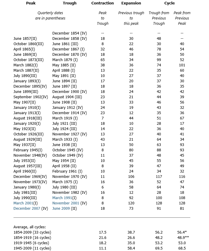
And the NBER site maintains a complete record of the US business cycle, dating back to the middle 1800’s, as shown in the following tables.

NBERbsdates

Periods of contraction, from peak to trough, are typically shorter than periods of expansion – or the movement from previous trough to the next peak.

Since World War II, the average length of the business cycle, variously measured from trough to trough or from peak to peak, is more than 5 years.

Focusing on the current situation, we are interested in the length of time from the previous peak of the business cycle in December 2007 to the next peak. The longest peak to peak period was over the prosperity of the 1990’s, and lasted more than 10 years (128 months).

So, it would be unusual if the peak of this current business cycle were much later than 2017-2018.

In terms of predicting turning points, matters are complicated by the fact that, unlike many European countries, the NBER does not define a recession in terms of two consecutive quarters of decline in real GDP.

Rather, a recession is a significant decline in economic activity spread across the economy, lasting more than a few months, normally visible in real GDP, real income, employment, industrial production, and wholesale-retail sales.

But just predicting the onset of two consecutive quarters of decline in real GDP is challenging. Indeed, the record of macroeconomic forecasting is very poor in this regard.

Part of the problem with the concept of a “cycle” in this context is the irregularity of the fluctuations derived by standard filters and methods.

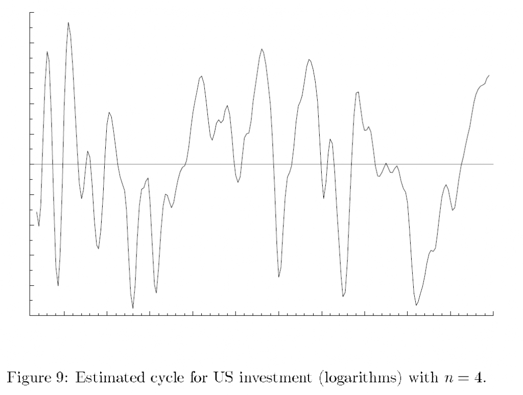
Harvey, for example, applies low band and pass Butterworth filters to US total investment and other macroeconomic series, deriving, at one pont, an investment “cycle” that looks like this.

Invcycle

So almost everything that makes a cycle useful in prediction is missing from this investment cycle. Thus, one cannot conclude that a turning point will occur, when the amplitude of the cycle is reached, since the amplitudes of these quasi-cycles vary considerably. Similarly, the “period” of the cycle is by no means fixed, but is basically stochastic, with a certain variance sometimes expressed as a “hyperparameter.” Only a certain quality of smoothness presents itself, and, of course, is a result of the filtering parameters that are applied.

In my opinion, industry cycles make a certain amount of sense, for particular industries, over particular spans of time. What I mean is that identification of such industry cycles improves predictability of the underlying series – be it sales or inventories or what have you.

The business cycle, on the other hand, is something of a metaphor, or maybe just an evocative phrase.

True, there are periods of economic contraction and periods of expansion.

But the extraction of macroeconomic cycles often does not improve predictability, because the fluctuations so identified are highly irregular from a number of different viewpoints.

I’ve sort of confirmed this is a quantitative sense by applying various cycle-extraction softwares to US real GDP to see whether any product or approach gave a hint that the Great Recession which began in 2008 would (a) occur, and (b) be as dramatic as it was. So far, no go.

And, of course, Ng points out that the Great Recession was fundamentally different than, say, recessions in the 1960’s sand 1970’s in that it was a balance sheet recession.

The Consumer Durable Inventory Cycle – Canary in the Coal Mine?

I’m continuing this week with posts about cycles and, inevitably, need to address one very popular method of extracting cycles from time series data – the Hodrick-Prescott (HP) filter.

Recently, I’ve been exploring inventory cycles, hoping to post something coherent.

I think I hit paydirt, as they say in gold mining circles.

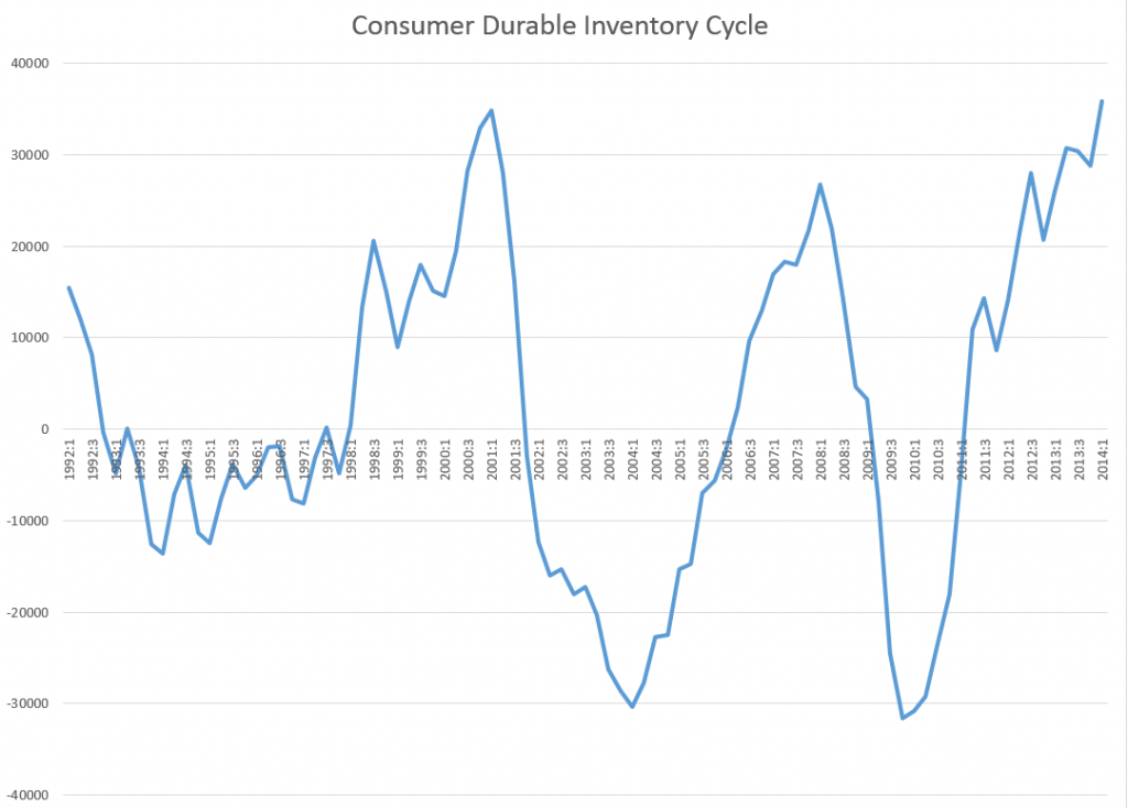
Here is the cycle component extracted from consumer durable inventories (not seasonally adjusted) from the Census manufacturing with a Hodrick-Prescott filter. I use a Matlab implementation here called hpfilter.

CDcycle

In terms of mechanics, the HP filter extracts the trend and cyclical component from a time series by minimizing an expression, as described by Wikipedia –

HPexp

What’s particularly interesting to me is that the peak of the two cycles in the diagram are spot-on the points at which the business cycle goes into recession – in 2001 and 2008.

Not only that, but the current consumer durable inventory cycle is credibly peaking right now and, based on these patterns, should go into a downward movement soon.

Of course, amplitudes of these cycles are a little iffy.

But the existence of a consumer durable cycle configured along these lines is consistent with the literature on inventory cycles, which emphasizes stockout-avoidance and relatively long pro-cyclical swings in inventories.

Semiconductor Cycles

I’ve been exploring cycles in the semiconductor, computer and IT industries generally for quite some time.

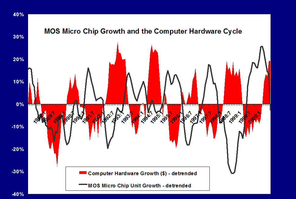
Here is an exhibit I prepared in 2000 for a magazine serving the printed circuit board industry.

semicycle

The data come from two sources – the Semiconductor Industry Association (SIA) World Semiconductor Trade Statistics database and the Census Bureau manufacturing series for computer equipment.

This sort of analytics spawned a spate of academic research, beginning more or less with the work of Tan and Mathews in Australia.

One of my favorites is a working paper released by DRUID – the Danish Research Unit for Industrial Dynamics called Cyclical Dynamics in Three Industries. Tan and Mathews consider cycles in semiconductors, computers, and what they call the flat panel display industry. They start with quoting “industry experts” and, specifically, some of my work with Economic Data Resources on the computer (PC) cycle. These researchers went on to publish in the Journal of Business Research and Technological Forecasting and Social Change in 2010. A year later in 2011, Tan published an interesting article on the sequencing of cyclical dynamics in semiconductors.

Essentially, the appearance of cycles and what I have called quasi-cycles or pseudo-cycles in the semiconductor industry and other IT categories, like computers, result from the interplay of innovation, investment, and pricing. In semiconductors, for example, Moore’s law – which everyone always predicts will fail at some imminent future point – indicates that continuing miniaturization will lead to periodic reductions in the cost of information processing. At some point in the 1980’s, this cadence was firmly established by introductions of new microprocessors by Intel roughly every 18 months. The enhanced speed and capacity of these microprocessors – the “central nervous system” of the computer – was complemented by continuing software upgrades, and, of course, by the movement to graphical interfaces with Windows and the succession of Windows releases.

Back along the supply chain, semiconductor fabs were retooling periodically to produce chips with more and more transitors per volume of silicon. These fabs were, simply put, fabulously expensive and the investment dynamics factors into pricing in semiconductors. There were famous gluts, for example, of memory chips in 1996, and overall the whole IT industry led the recession of 2001 with massive inventory overhang, resulting from double booking and the infamous Y2K scare.

Statistical Modeling of IT Cycles

A number of papers, summarized in Aubrey deploy VAR (vector autoregression) models to capture leading indicators of global semiconductor sales. A variant of these is the Bayesian VAR or BVAR model. Basically, VAR models sort of blindly specify all possible lags for all possible variables in a system of autoregressive models. Of course, some cutoff point has to be established, and the variables to be included in the VAR system have to be selected by one means or another. A BVAR simply reduces the number of possibilities by imposing, for example, sign constraints on the resulting coefficients, or, more ambitiously, employs some type of prior distribution for key variables.

Typical variables included in these models include:

  • WSTS monthly semiconductor shipments (now by subscription only from SIA)
  • Philadelphia semiconductor index (SOX) data
  • US data on various IT shipments, orders, inventories from M3
  • data from SEMI, the association of semiconductor equipment manufacturers

Another tactic is to filter out low and high frequency variability in a semiconductor sales series with something like the Hodrick-Prescott (HP) filter, and then conduct a spectral analysis.

Does the Semiconductor/Computer/IT Cycle Still Exist?

I wonder whether academic research into IT cycles is a case of “redoubling one’s efforts when you lose sight of the goal,” or more specifically, whether new configurations of forces are blurring the formerly fairly cleanly delineated pulses in sales growth for semiconductors, computers, and other IT hardware.

“Hardware” is probably a key here, since there have been big changes since the 1990’s and early years of this brave new century.

For one thing, complementarities between software and hardware upgrades seem to be breaking down. This began in earnest with the development of virtual servers – software which enabled many virtual machines on the same hardware frame, in part because the underlying circuitry was so massively powerful and high capacity now. Significant declines in the growth of sales of these machines followed on wide deployment of this software designed to achieve higher efficiencies of utilization of individual machines.

Another development is cloud computing. Running the data side of things is gradually being taken away from in-house IT departments in companies and moved over to cloud computing services. Of course, critical data for a company is always likely to be maintained in-house, but the need for expanding the number of big desktops with the number of employees is going away – or has indeed gone away.

At the same time, tablets, Apple products and Android machines, created a wave of destructive creation in people’s access to the Internet, and, more and more, for everyday functions like keeping calendars, taking notes, even writing and processing photos.

But note – I am not studding this discussion with numbers as of yet.

I suspect that underneath all this change it should be possible to identify some IT invariants, perhaps in usage categories, which continue to reflect a kind of pulse and cycle of activity.

Some Cycle Basics

A Fourier analysis is one of the first steps in analyzing cycles.

Take sunspots, for example,

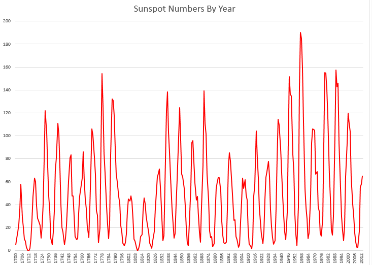
There are extensive historic records on the annual number of sunspots, dating back to 1700. The annual data shown in the following graph dates back to 1700, and is currently maintained by the Royal Belgium Observatory.

sunspots

This series is relatively stationary, although there may be a slight trend if you cut this span of data off a few years before the present.

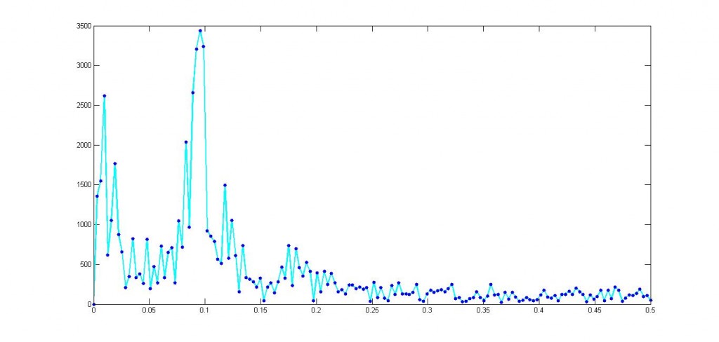
In any case, the kind of thing you get with a Fourier analysis looks like this.

spectralsunspots

This shows the power or importance of the cycles/year numbers, and maxes out at around 0.09.

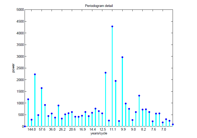
These data can be recalibrated into the following chart, which highlights the approximately 11 year major cycle in the sunspot numbers.

sunspotsperiodogramyr

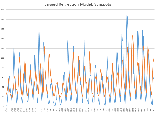
Now it’s possible to build a simple regression model with a lagged explanatory variable to make credible predictions. A lag of eleven years produces the following in-sample and out-of-sample fits. The regression is estimated over data to 1990, and, thus, the years 1991 through 2013 are out-of-sample.

LaggedModel

It’s obvious this sort of forecasting approach is not quite ready for prime-time television, even though it performs OK on several of the out-of-sample years after 1990.

But this exercise does highlight a couple of things.

First, the annual number of sunspots is broadly cyclical in this sense. If you try the same trick with lagged values for the US “business cycle” the results will be radically worse. At least with the sunspot data, most of the fluctuations have timing that is correctly predicted, both in-sample (1990 and before) and out-of-sample (1991-2013).

Secondly, there are stochastic elements to this solar activity cycle. The variation in amplitude is dramatic, and, indeed, the latest numbers coming in on sunspot activity are moving to much lower levels, even though the cycle is supposedly at its peak.

I’ve reviewed several papers on predicting the sunspot cycle. There are models which are more profoundly inspired by the possible physics involved – dynamo dynamics for example. But for my money there are basic models which, on a one-year-ahead basis, do a credible job. More on this forthcoming.

Cycles -1

I’d like  to focus on cycles in business and economic forecasting for the next posts.

The Business Cycle

“Cycles” – in connection with business and economic time series – evoke the so-called business cycle.

Immediately after World War II, Burns and Mitchell offered the following characterization –

Business cycles are a type of fluctuation found in the aggregate economic activity of nations that organize their work mainly in business enterprises: a cycle consists of expansions occurring at about the same time in many economic activities, followed by similarly general recessions, contractions, and revivals which merge into the expansion phase of the next cycle

Earlier, several types of business and economic cycles were hypothesized, based on their average duration. These included the 3 to 4 year Kitchin inventory investment cycle, a 7 to 11 year Juglar cycle associated with investment in machines, the 15 to 25 year Kuznets cycle, and the controversial Kondratieff cycle of from 48 to 60 years.

Industry Cycles

I have looked at industry cycles relating to movements of sales and prices in semiconductor and computer markets. While patterns may be changing, there is clear evidence of semi-regular pulses of activity in semiconductors and related markets. These stochastic cycles probably are connected with Moore’s Law and the continuing thrust of innovation and new product development.

Methods

Spectral analysis, VAR modeling, and standard autoregressive analysis are tools for developing evidence for time series cycles. STAMP, now part of the Oxmetrics suite of software, fits cycles with time-varying parameters.

Sometimes one hears of estimations in the time domain moving into the frequency domain. Time series, as normally graphed with time on the horizontal axis, are in the “time domain.” This is where VAR and autoregressive models operate. The frequency domain is where we get indications of the periodicity of cycles and semi-cycles in a time series.

Cycles as Artifacts

There is something roughly analogous to spurious correlation in regression analysis in the identification of cyclical phenomena in time series. Eugen Slutsky, a Russian mathematical economist and statistician, wrote a famous “unknown” paper on how moving averages of random numbers can create the illusion of cycles. Thus, if we add or average together elements of a time series in a moving window, it is easy to generate apparently cyclical phenomena. This can be demonstrated with the digits in the irrational number π, for example, since the sequence of digits 1 through 9 in its expansion is roughly random.

Significances

Cycles in business have sort of reassuring effect, it seems to me. And, of course, we are all very used to any number of periodic phenomena, ranging from the alternation of night and day, the phases of the moon, the tides, and the myriad of biological cycles.

As a paradigm, however, they probably used to be more important in business and economic circles, than they are today. There is perhaps one exception, and that is in rapidly changing high tech fields of which IT (information technology) is still in many respects a subcategory.

I’m looking forward to exploring some estimations, putting together some quantitative materials on this.

Links – late July

First post with my Android, so there are some minor items that need polishing – mainly how to embed links. It’s a complicated process, compared with MS Word and Windows.

In any case,  there are couple of fairly deep pieces here.

Enjoy.

A detailed exposé on how the market is rigged from a data-centric approach

We received trade execution reports from an active trader who wanted to know why his large orders almost never completely filled, even when the amount of stock advertised exceeded the number of shares wanted. For example, if 25,000 shares were at the best offer, and he sent in a limit order at the best offer price for 20,000 shares, the trade would, more likely than not, come back partially filled. In some cases, more than half of the amount of stock advertised (quoted) would disappear immediately before his order arrived at the exchange. This was the case, even in deeply liquid stocks such as Ford Motor Co (symbol F, market cap: $70 Billion, NYSE DMM is Barclays). The trader sent us his trade execution reports, and we matched up his trades with our detailed consolidated quote and trade data to discover that the mechanism described in Michael Lewis’s “Flash Boys” was alive and well on Wall Street.

This is just beautifully done. clean, simple, irrefutable. i hope it gets read far and wide. –Michael Lewis after reading this article

Did the Other Shoe Just Drop? Black Rock and PIMCO Sue Banks for $250 Billion. Any award this size would destabilize the banking system.

Rand Paul eyes tech-oriented donors, geeks in Bay Area.  The libertarian wedge in a liberal-dem stronghold.

Predictive analytics at World Cup  – Goldman Sachs does a big face plant, predicts Brazil would win. Importance of crowd-sourcing.

A Hands-on Lesson in Return Forecasting Models. I’ve almost never seen a longer blog post, and it ends up dissing the predictive models it exhaustively covers. But I think you will want to bookmark this one, and return to it for examples and ideas.


Yellen Yap: Silliness, Outright Lies, and Some Refreshingly Accurate Reporting. Point of concord between libertarian free market advocates and progressive-left commentators.


Video Friday – Andrew Ng’s Machine Learning Course

Well, I signed up for Andrew Ng’s Machine Learning Course at Stanford. It began a few weeks ago, and is a next generation to lectures by Ng circulating on YouTube. I’m going to basically audit the course, since I started a little late, but I plan to take several of the exams and work up a few of the projects. This course provides a broad introduction to machine learning, datamining, and statistical pattern recognition. Topics include: (i) Supervised learning (parametric/non-parametric algorithms, support vector machines, kernels, neural networks). (ii) Unsupervised learning (clustering, dimensionality reduction, recommender systems, deep learning). (iii) Best practices in machine learning (bias/variance theory; innovation process in machine learning and AI). The course will also draw from numerous case studies and applications, so that you’ll also learn how to apply learning algorithms to building smart robots (perception, control), text understanding (web search, anti-spam), computer vision, medical informatics, audio, database mining, and other areas. I like the change in format. The YouTube videos circulating on the web are lengthly, and involve Ng doing derivations on white boards. This is a more informal, expository format. Here is a link to a great short introduction to neural networks. Ngrobot Click on the link above this picture, since the picture itself does not trigger a YouTube. Ng’s introduction on this topic is fairly short, so here is the follow-on lecture, which starts the task of representing or modeling neural networks. I really like the way Ng approaches this is grounded in biology. I believe there is still time to sign up. Comment on Neural Networks and Machine Learning I can’t do much better than point to Professor Ng’s definition of machine learning – Machine learning is the science of getting computers to act without being explicitly programmed. In the past decade, machine learning has given us self-driving cars, practical speech recognition, effective web search, and a vastly improved understanding of the human genome. Machine learning is so pervasive today that you probably use it dozens of times a day without knowing it. Many researchers also think it is the best way to make progress towards human-level AI. In this class, you will learn about the most effective machine learning techniques, and gain practice implementing them and getting them to work for yourself. More importantly, you’ll learn about not only the theoretical underpinnings of learning, but also gain the practical know-how needed to quickly and powerfully apply these techniques to new problems. Finally, you’ll learn about some of Silicon Valley’s best practices in innovation as it pertains to machine learning and AI. And now maybe this is the future – the robot rock band.

Seasonal Adjustment – A Swirl of Controversies

My reading on procedures followed by the Bureau of Labor Statistics (BLS) and the Bureau of Economic Analysis (BLS) suggests some key US macroeconomic data series are in a profound state of disarray. Never-ending budget cuts to these “non-essential” agencies, since probably the time of Bill Clinton, have taken their toll.

For example, for some years now it has been impossible for independent analysts to verify or replicate real GDP and many other numbers issued by the BEA, since, only SA (seasonally adjusted) series are released, originally supposedly as an “economy measure.” Since estimates of real GDP growth by quarter are charged with political significance in an Election Year, this is a potential problem. And the problem is immediate, since the media naturally will interpret a weak 2nd quarter growth – less than, say, 2.9 percent – as a sign the economy has slipped into recession.

Evidence of Political Pressure on Government Statistical Agencies

John Williams has some fame with his site Shadow Government Statistics. But apart from extreme stances from time to time (“hyperinflation”), he does document the politicization of the BLS Consumer Price Index (CPI).

In a recent white paper called No. 515—PUBLIC COMMENT ON INFLATION MEASUREMENT AND THE CHAINED-CPI (C-CPI), Williams cites Katharine Abraham, former commissioner of the Bureau of Labor Statistics, when she notes,

“Back in the early winter of 1995, Federal Reserve Board Chairman Alan Greenspan testified before the Congress that he thought the CPI substantially overstated the rate of growth in the cost of living. His testimony generated a considerable amount of discussion. Soon afterwards, Speaker of the House Newt Gingrich, at a town meeting in Kennesaw, Georgia, was asked about the CPI and responded by saying, ‘We have a handful of bureaucrats who, all professional economists agree, have an error in their calculations. If they can’t get it right in the next 30 days or so, we zero them out, we transfer the responsibility to either the Federal Reserve or the Treasury and tell them to get it right.’”[v]

Abraham is quoted in newspaper articles as remembering sitting in Republican House Speaker Newt Gingrich’s office:

“ ‘He said to me, If you could see your way clear to doing these things, we might have more money for BLS programs.’ ” [vi]

The “things” in question were to move to quality adjustments for the basket of commodities used to calculate the CPI. The analogue today, of course, is the chained-CPI measure which many suggest is being promoted to slow cost-of-living adjustments in Social Security payments.

Of course, the “real” part in real GDP is linked with the CPI inflation outlook though a process supervised by the BEA.

Seasonal Adjustment Procedures for GDP

Here is a short video by Johnathan H. Wright, a young economist whose Unseasonal Seasonals? is featured in a recent issue of the Brookings Papers on Economic Activity.

Wright’s research is interesting to forecasters, because he concludes that algorithms for seasonally adjusting GDP should be selected based on their predictive performance.

Wright favors state-space models, rather than the moving-average techniques associated with the X-12 seasonal filters that date back to the 1980’s and even the 1960’s.

Given BLS methods of seasonal adjustment, seasonal and cyclical elements are confounded in the SA nonfarm payrolls series, due to sharp drops in employment concentrated in the November 2008 to March 2009 time window.

The upshot – initially this effect pushed reported seasonally adjusted nonfarm payrolls up in the first half of the year and down in the second half of the year, by slightly more than 100,000 in both cases…

One of his prime exhibits compares SA and NSA nonfarm payrolls, showing that,

The regular within-year variation in employment is comparable in magnitude to the effects of the 1990–1991 and 2001 recessions. In monthly change, the average absolute difference between the SA and NSA number is 660,000, which dwarfs the normal month-over-month variation in the SA data.
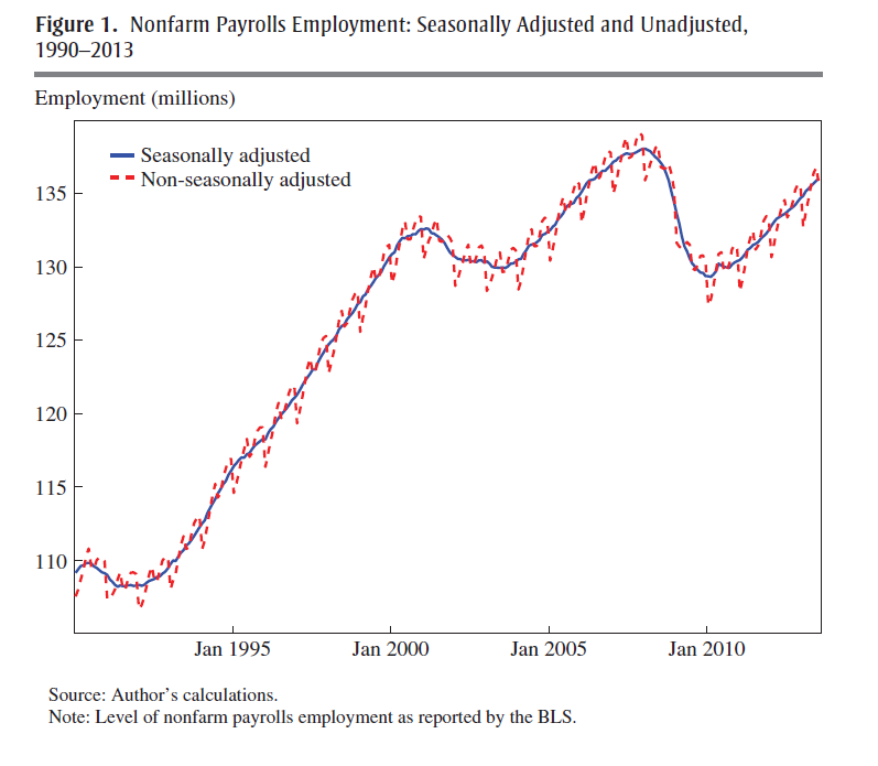
SEASnonseas

The basic procedure for this data and most releases since 2008-2009 follows what Wright calls the X-12 process.

The X-12 process focuses on certain types of centered moving averages with a fixed weights, based on distance from the central value.

A critical part of the X-12 process involves estimating the seasonal factors by taking weighted moving averages of data in the same period of different years. This is done by taking a symmetric n-term moving average of m-term averages, which is referred to as an n × m seasonal filter. For example, for n = m = 3, the weights are 1/3 on the year in question, 2/9 on the years before and after, and 1/9 on the two years before and after.16 The filter can be a 3 × 1, 3 × 3, 3 × 5, 3 × 9, 3 × 15, or stable filter. The stable filter averages the data in the same period of all available years. The default settings of the X-12…involve using a 3 × 3, 3 × 5, or 3 × 9 seasonal filter, depending on [various criteria]

Obviously, a problem arises at the beginning and at the end of the time series data. A work-around is to use an ARIMA model to extend the time series back and forward in time sufficiently to calculate these centered moving averages.

Wright shows these arbitrary weights and time windows lead to volatile seasonal adjustments, and that, predictively, the BEA and BLS would be better served with a state-space model based on the Kalman filter.

Loopy seasonal adjustment leads to controversy that airs on the web – such as this piece by Zero Hedge from 2012 which highlights the “ficititious” aspect of seasonal adjustments of highly tangible series, such as the number of persons employed –

What is very notable is that in January, absent BLS smoothing calculation, which are nowhere in the labor force, but solely in the mind of a few BLS employees, the real economy lost 2,689,000 jobs, while net of the adjustment, it actually gained 243,000 jobs: a delta of 2,932,000 jobs based solely on statistical assumptions in an excel spreadsheet!

To their credit, Census now documents an X-13ARIMA-SEATS Seasonal Adjustment Program with software incorporating elements of the SEATS procedure originally developed at the Bank of Spain and influenced by the state space models of Andrew Harvey.

Maybe Wright is getting some traction.

What Is The Point of Seasonal Adjustment?

You can’t beat the characterization, apparently from the German Bundesbank, of the purpose and objective of “seasonal adjustment.”

..seasonal adjustment transforms the world we live in into a world where no seasonal and working-day effects occur. In a seasonally adjusted world the temperature is exactly the same in winter as in the summer, there are no holidays, Christmas is abolished, people work every day in the week with the same intensity (no break over the weekend)..

I guess the notion is that, again, if we seasonally adjust and see a change in direction of a time series, why then it probably is a change in trend, rather than from special uses of a certain period.

But I think most of the professional forecasting community is beyond just taking their cue from a single number. It would be better to have the raw or not seasonally adjusted (NSA) series available with every press release, so analysts can apply their own models.

Analyzing Complex Seasonal Patterns

When time series data are available in frequencies higher than quarterly or monthly, many forecasting programs hit a wall in analyzing seasonal effects.

Researchers from the Australian Monash University published an interesting paper in the Journal of the American Statistical Association (JASA), along with an R program, to handle this situation – what can be called “complex seasonality.”

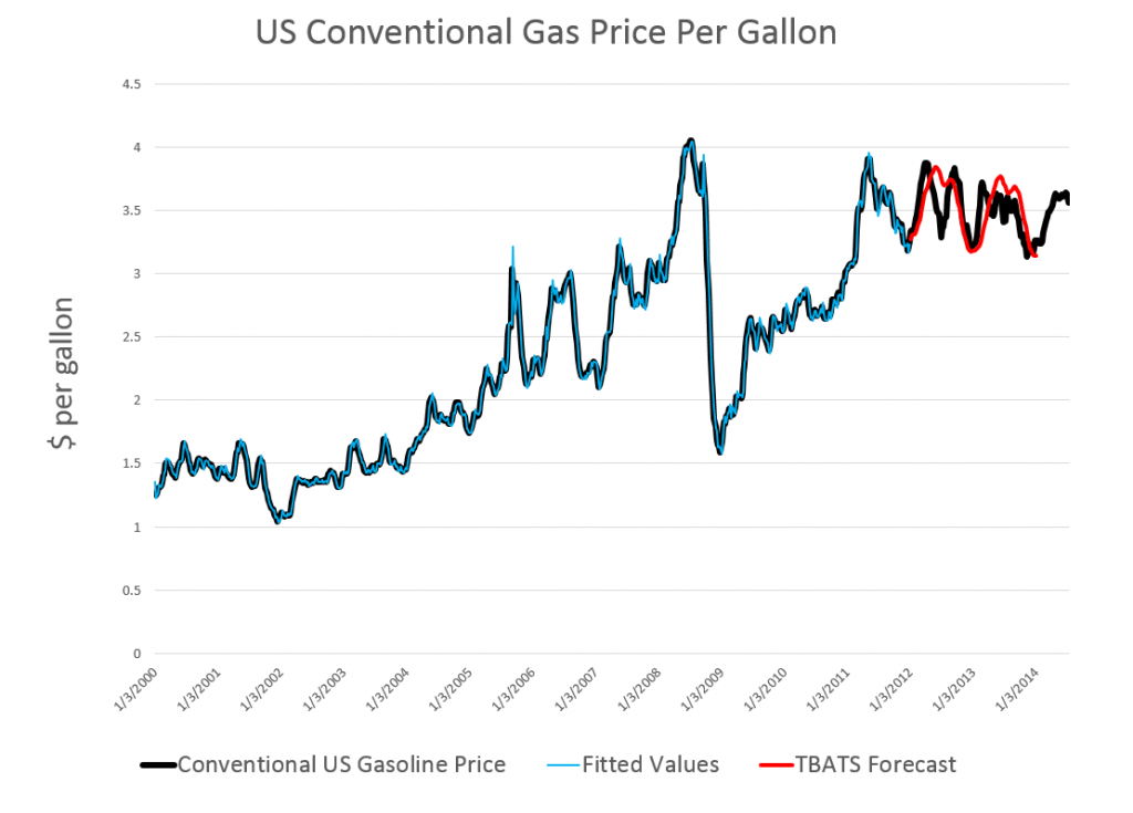
I’ve updated and modified one of their computations – using weekly, instead of daily, data on US conventional gasoline prices – and find the whole thing pretty intriguing.

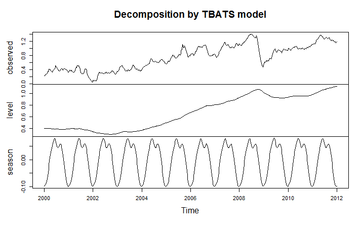
tbatschart

If you look at the color codes in the legend below the chart, it’s a little easier to read and understand.

Here’s what I did.

I grabbed the conventional weekly US gasoline prices from FRED. These prices are for “regular” – the plain vanilla choice at the pump. I established a start date of the first week in 2000, after looking the earlier data over. Then, I used tbats(.) in the Hyndman R Forecast package which readers familiar with this site know can be downloaded for use in the open source matrix programming language R.

Then, I established an end date for a time series I call newGP of the first week in 2012, forecasting ahead with the results of applying tbats(.) to the historic data from 2000:1 to 2012:1 where the second number refers to weeks which run from 1 to 52. Note that some data scrubbing is needed to shoehorn the gas price data into 52 weeks on a consistent basis. I averaged “week 53” with the nearest acceptable week (either 52 or 1 in the next year), and then got rid of the week 53’s.

The forecast for 104 weeks is shown by the solid red line in the chart above.

This actually looks promising, as if it might encode some useful information for, say, US transportation agencies.

A draft of the JASA paper is available as a PDF download. It’s called Forecasting time series with complex seasonal patterns using exponential smoothing and in addition to daily US gas prices, analyzes daily electricity demand in Turkey and bank call center data.

I’m only going part of the way to analyzing the gas price data, since I have not taken on daily data yet. But the seasonal pattern identified by tbats(.) from the weekly data is interesting and is shown below.

tbatsgasprice

The weekly frequency may enable us to “get inside” a mid-year wobble in the pattern with some precision. Judging from the out-of-sample performance of the model, this “wobble” can in some cases be accentuated and be quite significant.

Trignometric series fit to the higher frequency data extract the seasonal patterns in tbats(.), which also features other advanced features, such as a capability for estimating ARMA (autoregressive moving average) models for the residuals.

I’m not fully optimizing the estimation, but these results are sufficiently strong to encourage exploring the toggles and switches on the routine.

Another routine which works at this level of aggregation is the stlf(.) routine. This is uses STL decomposition described in some detail in Chapter 36 Patterns Discovery Based on Time-Series Decomposition in a collection of essays on data mining.

Thoughts

Good forecasting software elicits sort of addictive behavior, when initial applications of routines seem promising. How much better can the out-of-sample forecasts be made with optimization of the features of the routine? How well does the routine do when you look at several past periods? There is even the possibility of extracting further information from the residuals through bootstrapping or bagging at some point. I think there is no other way than exhaustive exploration.

The payoff to the forecaster is the amazement of his or her managers, when features of a forecast turn out to be spot-on, prescient, or what have you – and this does happen with good software. An alternative, for example, to the Hyndman R Forecast package is the program STAMP I also am exploring. STAMP has been around for many years with a version running – get this – on DOS, which appears to have had more features than the current Windows incarnation. In any case, I remember getting a “gee whiz” reaction from the executive of a regional bus district once, relating to ridership forecasts. So it’s fun to wring every possible pattern from the data.

Seasonal Sales Patterns – Stylized Facts

Seasonal sales patterns in the United States are more or less synchronized with Europe, Japan, China, and, to a lesser extent, the rest of the world.

Here are some stylized facts:

  1. Sales tend to peak at the end of the calendar year. This is the well-known “Christmas effect,” and is a strong enough factor to “cannibalize” demand, to an extent, at the first of the following year.
  2. Sales of final goods tend to be lower – in terms of growth rates and, in some cases, absolutely, in the first calendar quarter of the year.
  3. Supply chain effects, related to pulses of sales of final goods, can be identified for various lines of production depending on production lead times. Semiconductor orders, for example, tend to peak earlier than sales of consumer electronics, which are sharply influenced by the Christmas season.

To validate this picture, let me offer some evidence.

First, consider retail and food service sales data for the US, a benchmark of consumer activity – the recently discussed data downloaded from FRED.

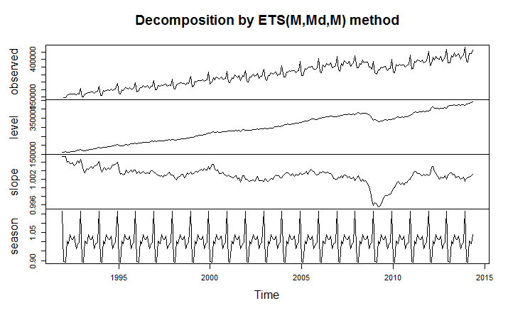
Applying the automatic model selection of the Hyndman R Forecast package, we get a decomposition of this time series into level, trend, and seasonals, as shown in the following diagram.

Rplotrs

The optimal exponential smoothing forecast model is a model with a damped trend and multiplicative seasonals.

If we look at the lower part of this diagram, we see that the seasonal factor for December – which is shown by the major peaks in the curve – is a multiple of more than 1.15. On the other hand, the immediately following month – January – shows a multiple of 0.9. These factors are multiplied into the product of the level and trend to get the sales for December and January. In other words, you can suppose that, roughly speaking, December retail sales will be 15 percent above trend, while January sales will be 90 percent of trend.

And, if you inspect this diagram in the lower panel carefully, you can detect the lull in late summer and fall in retail sales.

With “just-in-time” inventories and lean production models, actual production activity closely tracks these patterns in final demand – although it does take some lead time to produce stuff.

These stylized facts have not changed in their outlines since the ground-breaking research of Jeffrey Miron in the the late 1980’s. Miron refers to a worldwide seasonal cycle in aggregate economic activity whose major features are a fourth quarter boom in output.., a third quarter trough in manufacturing production, and a first quarter trough in all economic activity.

The Effects of Different Calendars – the Chinese New Year and Ramadan

The Gregorian calendar has achieved worldwide authority, and almost every country follows on the conventions of counting the year (currently 2014).

The Chinese calendar, however, is still important for determining the timing of festivals for Chinese communities around the world, and, especially, in China.

GRAPHICS TEMPLATE 2006

Similarly, the Islamic calendar governs the timing of important ritual periods and religious festivals – such as the month of Ramadan, which falls in June and July in 2014.

Because these festival periods overlap with multiple Gregorian months, there can be significant localized impacts on estimates of seasonal variation of economic activity.

Taiwanese researchers looking at this issue find significant holiday effects, related the fact that,

The three most important Chinese holidays, Chinese New Year, the Dragon-boat Festival, and Mid-Autumn Holiday have dates determined by a lunar calendar and move between two solar months. Consumption, production, and other economic behavior in countries with large Chinese population including Taiwan are strongly affected by these holidays. For example, production accelerates before lunar new year, almost completely stops during the holidays and gradually rises to an average level after the holidays.

Similarly, researchers in Pakistan consider the impacts of the Islamic festivals on standard macroeconomic and financial time series.