Category Archives: ordinary least squares (OLS) regression

Selecting Predictors

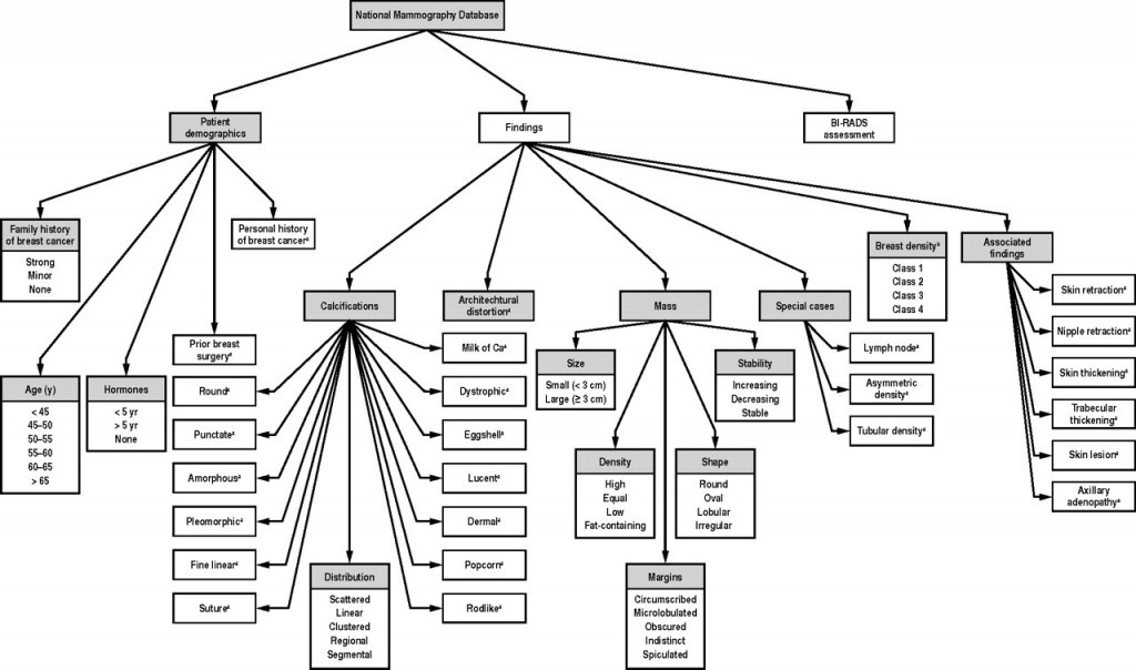
In a recent post on logistic regression, I mentioned research which developed diagnostic tools for breast cancer based on true Big Data parameters – notably 62,219 consecutive mammography records from 48,744 studies in 18,270 patients reported using the Breast Imaging Reporting and Data System (BI-RADS) lexicon and the National Mammography Database format between April 5, 1999 and February 9, 2004.

This research built a logistic regression model with 36 predictors, selected from the following information residing in the National Mammography Database (click to enlarge).

        breastcancertyp               

The question arises – are all these 36 predictors significant? Or what is the optimal model? How does one select the subset of the available predictor variables which really count?

This is the problem of selecting predictors in multivariate analysis – my focus for several posts coming up.

So we have a target variable y and set of potential predictors x={x1,x2,….,xn}. We are interested in discovering a predictive relationship, y=F(x*) where x* is some possibly proper subset of x. Furthermore, we have data comprising m observations on y and x, which in due time we will label with subscripts.

There are a range of solutions to this very real, very practical modeling problem.

Here is my short list.

  1. Forward Selection. Begin with no candidate variables in the model. Select the variable that boosts some goodness-of-fit or predictive metric the most. Traditionally, this has been R-Squared for an in-sample fit. At each step, select the candidate variable that increases the metric the most. Stop adding variables when none of the remaining variables are significant. Note that once a variable enters the model, it cannot be deleted.
  2. Backward Selection. This starts with the superset of potential predictors and eliminates variables which have the lowest score by some metric – traditionally, the t-statistic.
  3. Stepwise regression. This combines backward and forward selection of regressors.
  4. Regularization and Selection by means of the LASSO. Here is the classic article and here is a post, and here is a post in this blog on the LASSO.
  5. Information criteria applied to all possible regressions – pick the best specification by applying the Aikaike Information Criterion (AIC) or Bayesian Information Criterion (BIC) to all possible combinations of regressors. Clearly, this is only possible with a limited number of potential predictors.
  6. Cross-validation or other out-of-sample criteria applied to all possible regressions – Typically, the error metrics on the out-of-sample data cuts are averaged, and the lowest average error model is selected out of all possible combinations of predictors.
  7. Dimension reduction or data shrinkage with principal components. This is a many predictors formulation, whereby it is possible to reduce a large number of predictors to a few principal components which explain most of the variation in the data matrix.
  8. Dimension reduction or data shrinkage with partial least squares. This is similar to the PC approach, but employs a reduction to information from both the set of potential predictors and the dependent or target variable.

There certainly are other candidate techniques, but this is a good list to start with.

Wonderful topic, incidentally. Dives right into the inner sanctum of the mysteries of statistical science as practiced in the real world.

Let me give you the flavor of how hard it is to satisfy the classical criterion for variable selection, arriving at unbiased or consistent estimates of effects of a set of predictors.

And, really, the paradigmatic model is ordinary least squares (OLS) regression in which the predictive function F(.) is linear.

The Specification Problem

The problem few analysts understand is called specification error.

So assume that there is a true model – some linear expression in variables multiplied by their coefficients, possibly with a constant term added.

Then, we have some data to estimate this model.

Now the specification problem is that when predictors are not orthogonal, i.e. when they are correlated, leaving out a variable from the “true” specification imparts a bias to the estimates of coefficients of variables included in the regression.

This complications sequential methods of selecting predictors for the regression.

So in any case I will have comments forthcoming on methods of selecting predictors.
Hal Varian and the “New” Predictive Techniques

Big Data: New Tricks for Econometrics is, for my money, one of the best discussions of techniques like classification and regression trees, random forests, and penalized  regression (such as lasso, lars, and elastic nets) that can be found.

Varian, pictured aove, is emeritus professor in the School of Information, the Haas School of Business, and the Department of Economics at the University of California at Berkeley. Varian retired from full-time appointments at Berkeley to become Chief Economist at Google.

He also is among the elite academics publishing in the area of forecasting according to IDEAS!.

Big Data: New Tricks for Econometrics, as its title suggests, uses the wealth of data now being generated (Google is a good example) as a pretext for promoting techniques that are more well-known in machine learning circles, than in econometrics or standard statistics, at least as understood by economists.

First, the sheer size of the data involved may require more sophisticated 18 data manipulation tools. Second, we may have more potential predictors than appropriate for estimation, so we need to do some kind of variable selection. Third, large data sets may allow for more flexible relationships than simple linear models. Machine learning techniques such as decision trees, support vector machines, neural nets, deep learning and so on may allow for more effective ways to model complex relationships.

He handles the definitional stuff deftly, which is good, since there is not standardization of terms yet in this rapidly evolving field of data science or predictive analytics, whatever you want to call it.

Thus, “NoSQL” databases are

sometimes interpreted as meaning “not only SQL.” NoSQL databases are more primitive than SQL databases in terms of data manipulation capabilities but can handle larger amounts of data.

The essay emphasizes out-of-sample prediction and presents a nice discussion of k-fold cross validation.

1. Divide the data into k roughly equal subsets and label them by s =1; : : : ; k. Start with subset s = 1.

2. Pick a value for the tuning parameter.

3. Fit your model using the k -1 subsets other than subset s.

4. Predict for subset s and measure the associated loss.

5. Stop if s = k, otherwise increment s by 1 and go to step 2.

Common choices for k are 10, 5, and the sample size minus 1 (“leave one out”). After cross validation, you end up with k values of the tuning parameter and the associated loss which you can then examine to choose an appropriate value for the tuning parameter. Even if there is no tuning parameter, it is useful to use cross validation to report goodness-of-t measures since it measures out-of-sample performance which is what is typically of interest.

Varian remarks that Test-train and cross validation, are very commonly used in machine learning and, in my view, should be used much more in economics, particularly when working with large datasets

But this essay is by no means methodological, and presents several nice worked examples, showing how, for example, regression trees can outperform logistic regression in analyzing survivors of the sinking of the Titanic – the luxury ship, and how several of these methods lead to different imputations of significance to the race factor in the Boston Housing Study.

The essay also presents easy and good discussions of bootstrapping, bagging, boosting, and random forests, among the leading examples of “new” techniques – new to economists.

For the statistics wonks, geeks, and enthusiasts among readers, here is a YouTube presentation of the paper cited above with extra detail.


Forecasting in Data-limited Situations – A New Day

Over the Holidays – while frustrated in posting by a software glitch – I looked at the whole “shallow data issue” in light of  a new technique I’ve learned called bagging.

Bottom line, using spreadsheet simulations, I can show bagging radically reduces out-of-sample forecast error, in a situation typical for a lot business forecasting – where there are just a few workable observations, quite a few candidate drivers or explanatory variables, and a lot of noise in the data.

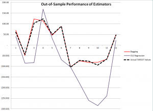
Here is a comparison of the performance of OLS regression and bagging with out-of-sample data generated with the same rules which create the “sample data” in the example spreadsheet shown below.

SmallDATAgraphcomp

The contrast is truly stark. Although, as we will see, the ordinary least squares (OLS) regression has an R2 or “goodness of fit” of 0.99, it does not generalize well out-of-sample, producing the purple line in the graph with 12 additional cases or observations. Bagging the original sample 200 times and re-estimating OLS regression on the bagged samples, then averaging the regression constants and coefficients, produces a much tighter fit on these out-of-sample observations.

Example Spreadsheet

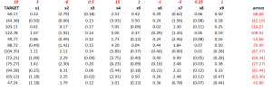
The spreadsheet below illustrates 12 “observations” on a  TARGET or dependent variable and nine (9) explanatory variables, x1 through x9.

SmallDATA1

The top row with numbers in red lists the “true” values of these explanatory variables or drivers, and the column of numbers in red on the far right are the error terms (which are generated by a normal distribution with zero mean and standard deviation of 50).

So if we multiply 3 times 0.22 and add -6 times -2.79 and so forth, adding 68.68 at the end, we get the first value of the TARGET variable 60.17.

While this example is purely artificial, an artifact, one can imagine that these numbers are first differences – that is the current value of a variable minus its preceding value. Thus, the TARGET variable might record first differences in sales of a product quarter by quarter. And we suppose forecasts for  x1 through x9 are available, although not shown above. In fact, they are generated in simulations with the same generating mechanisms utilized to create the sample.

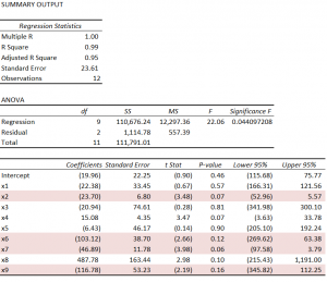
Using the simplest multivariate approach, the ordinary least squares (OLS) regression, displayed in the Excel format, is –

SmallDATAreg

There’s useful information in this display, often the basis of a sort of “talk-through” the regression result. Usually, the R2 is highlighted, and it is terrific here, “explaining” 99 percent of the variation in the data, in, that is, the 12 in-sample values for the TARGET variable. Furthermore, four explanatory variables have statistically significant coefficients, judged by their t-statistics – x2, x6, x7, and x9. These are highlighted in a kind of purple in the display.

Of course, the estimated values of x1 through x9 are, for the most part, numerically quite different than the true values of the constant term and coefficients {10, 3, -6, 0.5, 15, 1, -1, -5, 0.25, 1}. Nevertheless, because of the large variances or standard errors of the estimates, as noted above some estimated coefficients are within a 95 percent confidence interval of these true values. It’s just that the confidence intervals are very wide.

The in-sample predicted values are accurate, generally speaking. These loopy coefficient estimates essentially balance one another off in-sample.

But it’s not the in-sample performance we are interested in, but the out-of-sample performance. And we want to compare the out-of-sample performance of this OLS regression estimate with estimates of the coefficients and TARGET variable produced by ridge regression and bagging.

Bagging

Bagging [bootstrap aggregating] was introduced by Breiman in the 1990’s to reduce the variance of predictors. The idea is that you take N bootstrap samples of the original data, and with each of these samples, estimate your model, creating, in the end, an ensemble prediction.

Bootstrap sampling draws random samples with replacement from the original sample, creating other samples of the same size. With 12 cases or observations on the TARGET and explanatory variables there are a large number of possible random samples of these 12 cases drawn with replacement; in fact, given nine explanatory variables and the TARGET variable, there are 129  or somewhat more than 5 billion distinct samples, 12 of which, incidentally, are comprised of exactly the same case drawn repeatedly from the original sample.

A primary application of bagging has been in improving the performance of decision trees and systems of classification. Applications to regression analysis seem to be more or less an after-thought in the literature, and the technique does not seem to be in much use in applied business forecasting contexts.

Thus, in the spreadsheet above, random draws with replacement are taken of the twelve rows of the spreadsheet (TARGET and drivers) 200 times, creating 200 samples. An ordinary least squares regression is estimated over each regression, and the constant and parameter estimates are averaged at the end of the process.

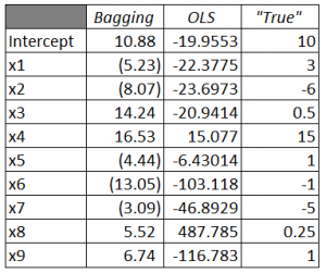
Here is a comparison of the estimated coefficients from Bagging and OLS, compared with the true values.

BaggingTable

There’s still variation of the parameter estimates from the true values with bagging, but the variance of the error process (50) is, by design, high. For example, most of the value of TARGET is from the error process, so this is noisy data.

Discussion

Some questions. For example – Are there specific features of the problem presented here which tip the results markedly in favor of bagging? What are the criteria for determining whether bagging will improve regression forecasts? Another question regards the ease or difficulty of bagging regressions in Excel.

The criterion for bagging to deliver dividends is basically parameter instability over the sample. Thus, in the problem here, deleting any observation from the 12 cases and re-estimating the regression results in big changes to estimated parameters. The basic reason is the error terms constitute by far the largest contribution to the value of TARGET for each case.

In practical forecasting, this criterion, which not very clearly defined, can be explored, and then comparisons with regard to actual outcomes can be studied. Thus, estimate the bagged regression forecast,  wait a period, and compare bagged and simple OLS forecasts. Substantial improvement in forecast accuracy, combined with parameter instability in the sample, would seem to be a smoking gun.

Apart from the large contribution of the errors or residuals to the values of TARGET, the other distinctive feature of the problem presented here is the large number of predictors in comparison with the number of cases or observations. This, in part, accounts for the high coefficient of determination or R2, and also suggests that the close in-sample fit and poor out-of-sample performance are probably related to “over-fitting.”