Category Archives: variable selection

Primer on Method – Some Perspectives from 2014

As Hal Varian writes in his popular Big Data: New Tricks for Econometrics the wealth of data now available to researchers demands new techniques of analysis.

In particular, often there is the problem of “many predictors.” In classic regression, the number of observations is assumed to exceed the number of explanatory variables. This obviously is challenged in the Big Data context.

Variable selection procedures are one tactic in this situation.

Readers may want to consult the post Selecting Predictors. It has my list of methods, as follows:

  1. Forward Selection. Begin with no candidate variables in the model. Select the variable that boosts some goodness-of-fit or predictive metric the most. Traditionally, this has been R-Squared for an in-sample fit. At each step, select the candidate variable that increases the metric the most. Stop adding variables when none of the remaining variables are significant. Note that once a variable enters the model, it cannot be deleted.
  2. Backward Selection. This starts with the superset of potential predictors and eliminates variables which have the lowest score by some metric – traditionally, the t-statistic.
  3. Stepwise regression. This combines backward and forward selection of regressors.
  4. Regularization and Selection by means of the LASSO. Here is the classic article and here is a post in this blog on the LASSO.
  5. Information criteria applied to all possible regressions – pick the best specification by applying the Aikaike Information Criterion (AIC) or Bayesian Information Criterion (BIC) to all possible combinations of regressors. Clearly, this is only possible with a limited number of potential predictors.
  6. Cross-validation or other out-of-sample criteria applied to all possible regressions– Typically, the error metrics on the out-of-sample data cuts are averaged, and the lowest average error model is selected out of all possible combinations of predictors.
  7. Dimension reduction or data shrinkage with principal components. This is a many predictors formulation, whereby it is possible to reduce a large number of predictors to a few principal components which explain most of the variation in the data matrix.
  8. Dimension reduction or data shrinkage with partial least squares. This is similar to the PC approach, but employs a reduction to information from both the set of potential predictors and the dependent or target variable.

Some more supporting posts are found here, usually with spreadsheet-based “toy” examples:

Three Pass Regression Filter, Partial Least Squares and Principal Components, Complete Subset Regressions, Variable Selection Procedures – the Lasso, Kernel Ridge Regression – A Toy Example, Dimension Reduction With Principal Components, bootstrapping, exponential smoothing, Estimation and Variable Selection with Ridge Regression and the LASSO

Plus one of the nicest infographics on machine learning – a related subject – is developed by the Australian blog Machine Learning Mastery.

MachineLearning

Complete Subset Regressions

A couple of years or so ago, I analyzed a software customer satisfaction survey, focusing on larger corporate users. I had firmagraphics – specifying customer features (size, market segment) – and customer evaluation of product features and support, as well as technical training. Altogether, there were 200 questions that translated into metrics or variables, along with measures of customer satisfaction. Altogether, the survey elicited responses from about 5000 companies.

Now this is really sort of an Ur-problem for me. How do you discover relationships in this sort of data space? How do you pick out the most important variables?

Since researching this blog, I’ve learned a lot about this problem. And one of the more fascinating approaches is the recent development named complete subset regressions.

And before describing some Monte Carlo exploring this approach here, I’m pleased Elliot, Gargano, and Timmerman (EGT) validate an intuition I had with this “Ur-problem.” In the survey I mentioned above, I calculated a whole bunch of univariate regressions with customer satisfaction as the dependent variable and each questionnaire variable as the explanatory variable – sort of one step beyond calculating simple correlations. Then, it occurred to me that I might combine all these 200 simple regressions into a predictive relationship. To my surprise, EGT’s research indicates that might have worked, but not be as effective as complete subset regression.

Complete Subset Regression (CSR) Procedure

As I understand it, the idea behind CSR is you run regressions with all possible combinations of some number r less than the total number n of candidate or possible predictors. The final prediction is developed as a simple average of the forecasts from these regressions with r predictors. While some of these regressions may exhibit bias due to specification error and covariance between included and omitted variables, these biases tend to average out, when the right number r < n is selected.

So, maybe you have a database with m observations or cases on some target variable and n predictors.

And you are in the dark as to which of these n predictors or potential explanatory variables really do relate to the target variable.

That is, in a regression y = β01 x1 +…+βn xn some of the beta coefficients may in fact be zero, since there may be zero influence between the associated xi and the target variable y.

Of course, calling all the n variables xi i=1,…n “predictor variables” presupposes more than we know initially. Some of the xi could in fact be “irrelevant variables” with no influence on y.

In a nutshell, the CSR procedure involves taking all possible combinations of some subset r of the n total number of potential predictor variables in the database, and mapping or regressing all these possible combinations onto the dependent variable y. Then, for prediction, an average of the forecasts of all these regressions is often a better predictor than can be generated by other methods – such as the LASSO or bagging.

EGT offer a time series example as an empirical application. based on stock returns, quarterly from 1947-2010 and twelve (12) predictors. The authors determine that the best results are obtained with a small subset of the twelve predictors, and compare these results with ridge regression, bagging, Lasso and Bayesian Model Averaging.

The article in The Journal of Econometrics is well-worth purchasing, if you are not a subscriber. Otherwise, there is a draft in PDF format from 2012.

The combination of n things taken r at a time is n!/[(n-r)!(r!)] and increases faster than exponentially, as n increases. For large n, accordingly, it is necessary to sample from the possible set of combinations – a procedure which still can generate improvements in forecast accuracy over a “kitchen sink” regression (under circumstances further delineated below). Otherwise, you need a quantum computer to process very fat databases.

When CSR Works Best – Professor Elloitt

I had email correspondence with Professor Graham Elliott, one of the co-authors of the above-cited paper in the Journal of Econometrics.

His recommendation is that CSR works best with when there are “weak predictors” sort of buried among a superset of candidate variables,

If a few (say 3) of the variables have large coefficients such as that they result in a relatively large R-square for the prediction regression when they are all included, then CSR is not likely to be the best approach. In this case model selection has a high chance of finding a decent model, the kitchen sink model is not all that much worse (about 3/T times the variance of the residual where T is the sample size) and CSR is likely to be not that great… When there is clear evidence that a predictor should be included then it should be always included…, rather than sometimes as in our method. You will notice that in section 2.3 of the paper that we construct properties where beta is local to zero – what this math says in reality is that we mean the situation where there is very little clear evidence that any predictor is useful but we believe that some or all have some minor predictive ability (the stock market example is a clear case of this). This is the situation where we expect the method to work well. ..But at the end of the day, there is no perfect method for all situations.

I have been toying with “hidden variables” and, then, measurement error in the predictor variables in simulations that further validate Graham Elliot’s perspective that CSR works best with “weak predictors.”

Monte Carlo Simulation

Here’s the spreadsheet for a relevant simulation (click to enlarge).
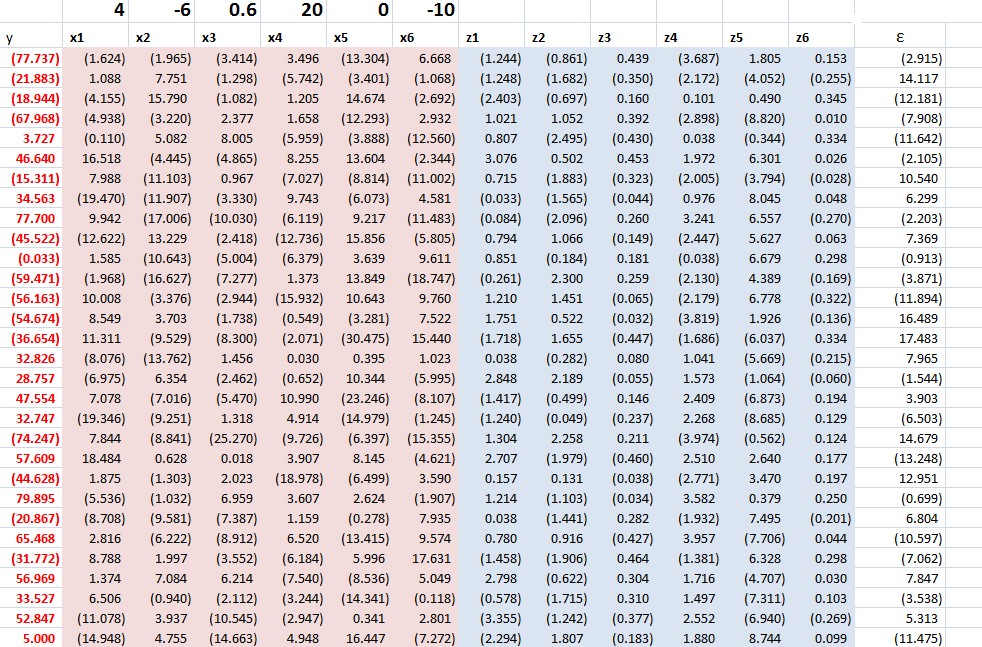
CSRTable

It is pretty easy to understand this spreadsheet, but it may take a few seconds. It is a case of latent variables, or underlying variables disguised by measurement error.

The z values determine the y value. The z values are multiplied by the bold face numbers in the top row, added together, and then the epsilon error ε value is added to this sum of terms to get each y value. You have to associate the first bold face coefficient with the first z variable, and so forth.

At the same time, an observer only has the x values at his or her disposal to estimate a predictive relationship.

These x variables are generated by adding a Gaussian error to the corresponding value of the z variables.

Note that z5 is an irrelevant variable, since its coefficient loading is zero.

This is a measurement error situation (see the lecture notes on “measurement error in X variables” ).

The relationship with all six regressors – the so-called “kitchen-sink” regression – clearly shows a situation of “weak predictors.”

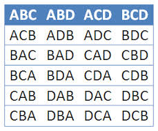
I consider all possible combinations of these 6 variables, taken 3 at a time, or 20 possible distinct combinations of regressors and resulting regressions.

In terms of the mechanics of doing this, it’s helpful to set up the following type of listing of the combinations.
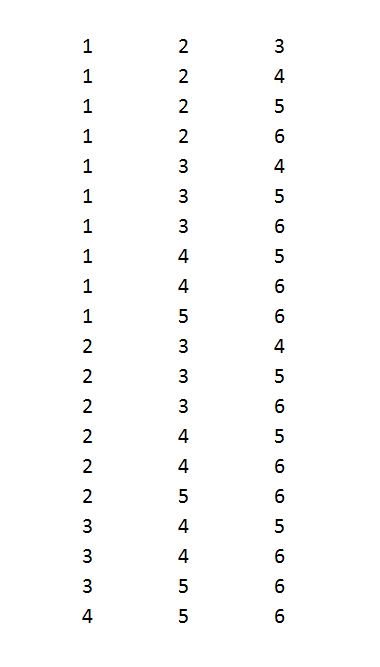
Combos

Each digit in the above numbers indicates a variable to include. So 123 indicates a regression with y and x1, x2, and x3. Note that writing the combinations in this way so they look like numbers in order of increasing size can be done by a simple algorithm for any r and n.

And I can generate thousands of cases by allowing the epsilon ε values and other random errors to vary.

In the specific run above, the CSR average soundly beats the mean square error (MSE) of this full specification in forecasts over ten out-of-sample values. The MSE of the kitchen sink regression, thus, is 2,440 while the MSE of the regression specifying all six regressors is 2653. It’s also true that picking the lowest within-sample MSE among the 20 possible combinations for k = 3 does not produce a lower MSE in the out-of-sample run.

This is characteristics of results in other draws of the random elements. I hesitate to characterize the totality without further studying the requirements for the number of runs, given the variances, and so forth.

I think CSR is exciting research, and hope to learn more about these procedures and report in future posts.

Variable Selection Procedures – The LASSO

The LASSO (Least Absolute Shrinkage and Selection Operator) is a method of automatic variable selection which can be used to select predictors X* of a target variable Y from a larger set of potential or candidate predictors X.

Developed in 1996 by Tibshirani, the LASSO formulates curve fitting as a quadratic programming problem, where the objective function penalizes the absolute size of the regression coefficients, based on the value of a tuning parameter λ. In doing so, the LASSO can drive the coefficients of irrelevant variables to zero, thus performing automatic variable selection.

This post features a toy example illustrating tactics in variable selection with the lasso. The post also dicusses the issue of consistency – how we know from a large sample perspective that we are honing in on the true set of predictors when we apply the LASSO.

My take is a two-step approach is often best. The first step is to use the LASSO to identify a subset of potential predictors which are likely to include the best predictors. Then, implement stepwise regression or other standard variable selection procedures to select the final specification, since there is a presumption that the LASSO “over-selects” (Suggested at the end of On Model Selection Consistency of Lasso).

Toy Example

The LASSO penalizes the absolute size of the regression coefficients, based on the value of a tuning parameter λ. When there are many possible predictors, many of which actually exert zero to little influence on a target variable, the lasso can be especially useful in variable selection.

For example, generate a batch of random variables in a 100 by 15 array – representing 100 observations on 15 potential explanatory variables. Mean-center each column. Then, determine coefficient values for these 15 explanatory variables, allowing several to have zero contribution to the dependent variable. Calculate the value of the dependent variable y for each of these 100 cases, adding in a normally distributed error term.

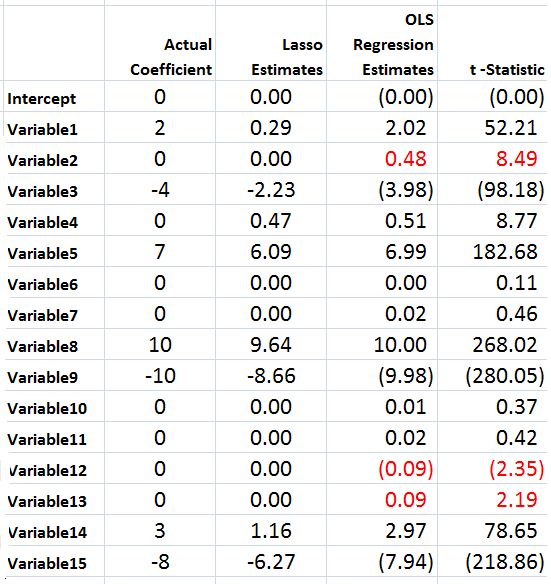
The following Table illustrates something of the power of the lasso.

LassoSS

Using the Matlab lasso procedure and a lambda value of 0.3, seven of the eight zero coefficients are correctly identified. The OLS regression estimate, on the other hand, indicates that three of the zero coefficients are nonzero at a level of 95 percent statistical significance or more (magnitude of the t-statistic > 2).

Of course, the lasso also shrinks the value of the nonzero coefficients. Like ridge regression, then, the lasso introduces bias to parameter estimates, and, indeed, for large enough values of lambda drives all coefficient to zero.

Note OLS can become impossible, when the number of predictors in X* is greater than the number of observations in Y and X. The LASSO, however, has no problem dealing with many predictors.

Real World Examples

For a recent application of the lasso, see the Dallas Federal Reserve occasional paper Hedge Fund Dynamic Market Stability. Note that the lasso is used to identify the key drivers, and other estimation techniques are employed to hone in on the parameter estimates.

For an application of the LASSO to logistic regression in genetics and molecular biology, see Lasso Logistic Regression, GSoft and the Cyclic Coordinate Descent Algorithm, Application to Gene Expression Data. As the title suggests, this illustrates the use of the lasso in logistic regression, frequently utilized in biomedical applications.

Formal Statement of the Problem Solved by the LASSO

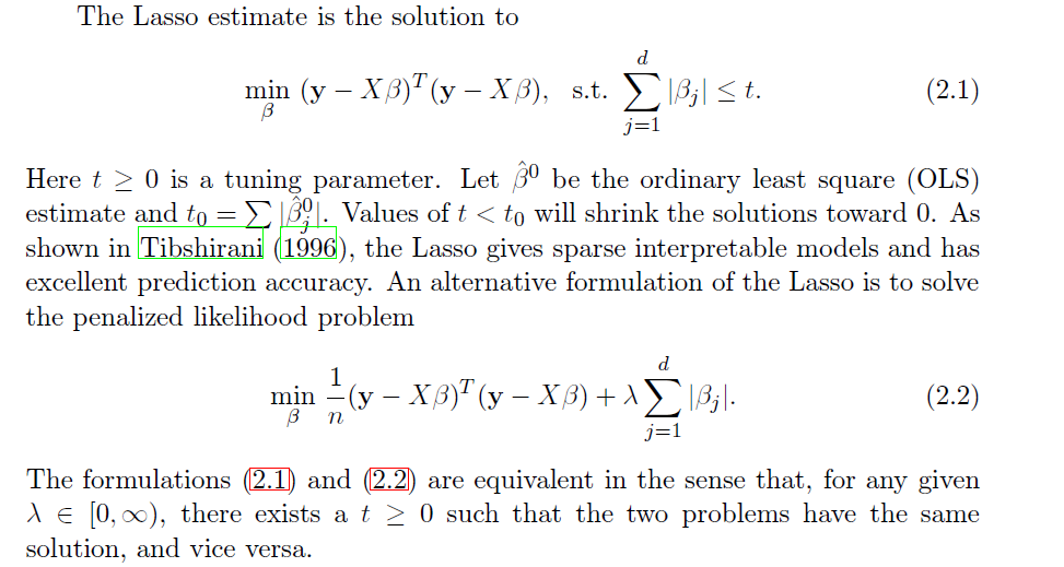
The objective function in the lasso involves minimizing the residual sum of squares, the same entity figuring in ordinary least squares (OLS) regression, subject to a bound on the sum of the absolute value of the coefficients. The following clarifies this in notation, spelling out the objective function.

LassoDerivation

LassoDerivation2

The computation of the lasso solutions is a quadratic programming problem, tackled by standard numerical analysis algorithms. For an analytical discussion of the lasso and other regression shrinkage methods, see the outstanding free textbook The Elements of Statistical Learning by Hastie, Tibshirani, and Friedman.

The Issue of Consistency

The consistency of an estimator or procedure concerns its large sample characteristics. We know the LASSO produces biased parameter estimates, so the relevant consistency is whether the LASSO correctly predicts which variables from a larger set are in fact the predictors.

In other words, when can the LASSO select the “true model?”

Now in the past, this literature is extraordinarily opaque, involving something called the Irrepresentable Condition, which can be glossed as –

almost necessary and sufficient for Lasso to select the true model both in the classical fixed p setting and in the large p setting as the sample size n gets large…This Irrepresentable Condition, which depends mainly on the covariance of the predictor variables, states that Lasso selects the true model consistently if and (almost) only if the predictors that are not in the true model are “irrepresentable” (in a sense to be clarified) by predictors that are in the true model.

Fortunately a ray of light has burst through with Assumptionless Consistency of the Lasso by Chatterjee. Apparently, the LASSO selects the true model almost always – with minimal side assumptions – providing we are satisfied with the prediction error criterion – the mean square prediction error – employed in Tibshirani’s original paper.

Finally, cross-validation is typically used to select the tuning parameter λ, and is another example of this procedure highlighted by Varian’s recent paper.