Tag Archives: automatic forecast programs

ARIMA models, Box Jenkins forecasts, business trends, retail trends, seasonal variation

Forecasting Holiday Retail Sales

December 14, 2014 Clive Jones

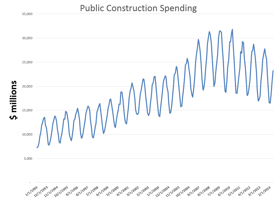
Holiday retail sales are a really “spikey” time series, illustrated by the following graph (click to enlarge).

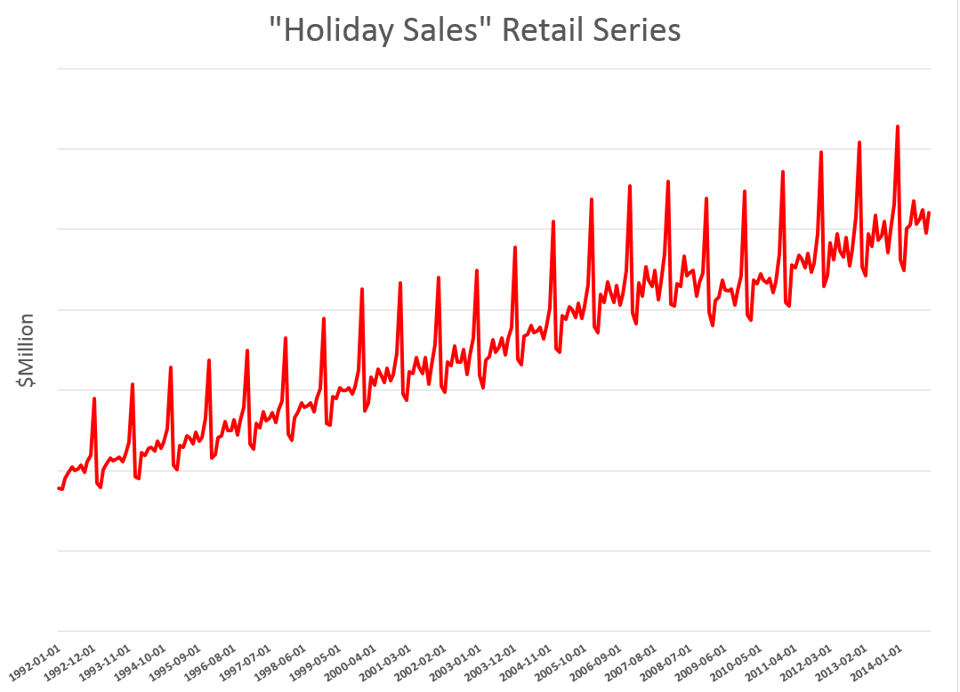
These are monthly data from FRED and are not seasonally adjusted.

Following the National Retail Federation (NRF) convention, I define holiday retail sales to exclude retail sales by automobile dealers, gasoline stations and restaurants. The graph above includes all months of the year, but we can again follow the NRF convention and define “sales from the Holiday period” as being November and December sales.

Current Forecasts

The National Retail Federation (NRF) issues its forecast for the Holiday sales period in late October.

This year, it seems they were a tad optimistic, opting for

..sales in November and December (excluding autos, gas and restaurant sales) to increase a healthy 4.1 percent to $616.9 billion, higher than 2013’s actual 3.1 percent increase during that same time frame.

As the news release for this forecast observed, this would make the Holiday Season 2014 the first time in many years to see more than 4 percent growth – comparing to the year previous holiday periods.

The NRF is still holding to its bet (See https://nrf.com/news/retail-sales-increase-06-percent-november-line-nrf-holiday-forecast), noting that November 2014 sales come in around 3.2 percent over the total for November in 2013.

This means that December sales have to grow by about 4.8 percent on a month-over-year-previous-month basis to meet the overall, two month 4.1 percent growth.

You don’t get to this number by applying univariate automatic forecasting software. Forecast Pro, for example, suggests overall year-over-year growth this holiday season will be more like 3.3 percent, or a little lower than the 2013 growth of 3.7 percent.

Clearly, the argument for higher growth is the extra cash in consumer pockets from lower gas prices, as well as the strengthening employment outlook.

The 4.1 percent growth, incidentally, is within the 97.5 percent confidence interval for the Forecast Pro forecast, shown in the following chart.

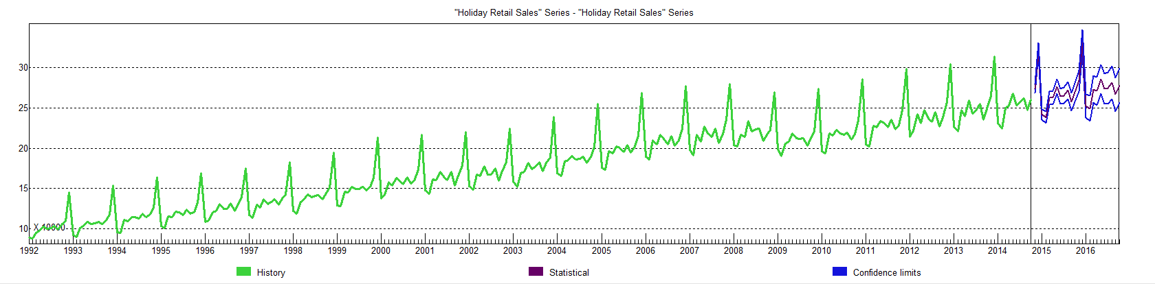
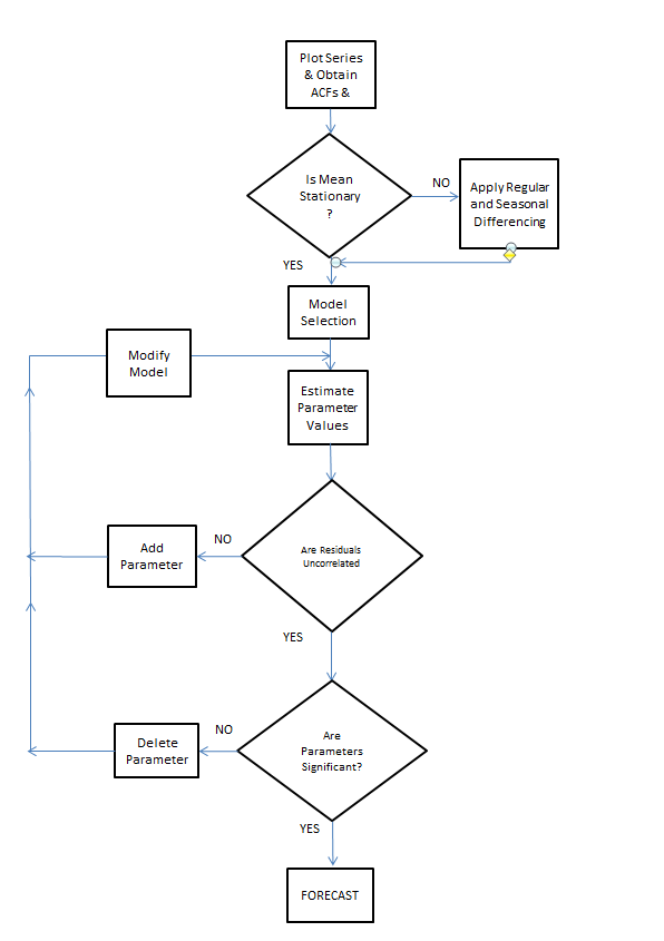
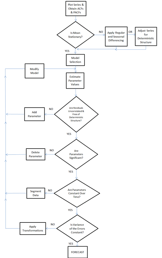
This forecast follows from a Box-Jenkins model with the parameters –

ARIMA(1, 1, 3)*(0, 1, 2)

In other words, Forecast Pro differences the “Holiday Sales” Retail Series and finds moving average and autoregressive terms, as well as seasonality. For a crib on ARIMA modeling and the above notation, a Duke University site is good.

I guess we will see which is right – the NRF or Forecast Pro forecast.

Components of US Retail Sales

The following graphic shows the composition of total US retail sales, and the relative sizes of the main components.

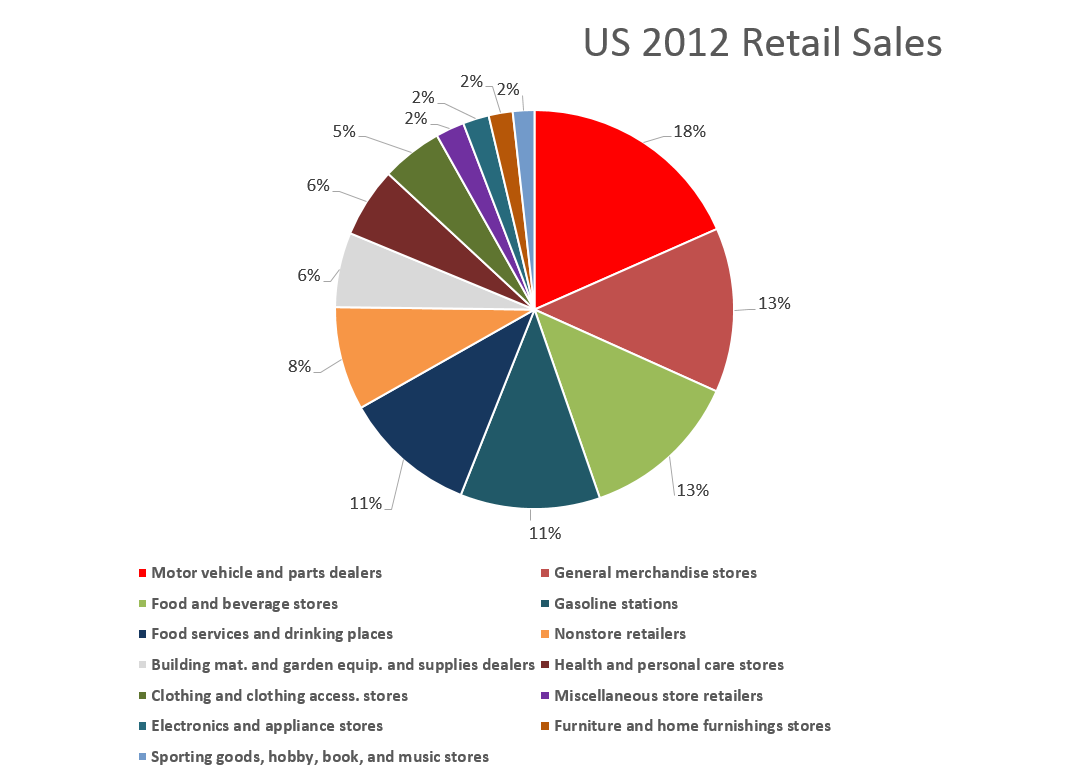
Retail and food service sales totaled around $5 trillion in 2012. Taking out motor vehicle and parts dealers, gas stations, and food services and drinking places considerably reduces the size of the relevant Holiday retail time series.

Forecasting Issues and Opportunities

I have not yet done the exercise, but it would be interesting to forecast the individual series in the above pie chart, and compare the sum of those forecasts with a forecast of the total.

For example, if some of the component series are best forecast with exponential smoothing, while others are best forecast with Box-Jenkins time series models, aggregation could be interesting.

Of course, in 2007-09, application of univariate methods would have performed poorly. What we cry out for here is a multivariate model, perhaps based on the Kalman filter, which specifies leading indicators. That way, we could get one or two month ahead forecasts without having to forecast the drivers or explanatory variables.

In any case, barring unforeseen catastrophes, this Holiday Season should show comfortable growth for retailers, especially online retail (more on that in a subsequent post.)

Heading picture from New York Times

accuracy of forecasts, analytical software, automatic forecasting software, exponential smoothing

Exponential Smoothing – Black Box Examples

July 7, 2014 Clive Jones

The reason why most people would be interested in and concerned with exponential smoothing (ES) is that it is an effective forecasting technique.

So, with that in mind, I want to discuss two automatic forecasting programs – Forecast Pro and Hyndman’s Forecast program for R – applied to a monthly time series for public construction spending in the US. I do this more or less “black box” in that I am not spending a lot of time on the underlying theory – which is basically a state space model framework – but focus on the process of getting the forecasts and their comparison.

I am testing these programs with a backcasting exercise. Thus, the data for this time series, available from FRED begin January 1993 and extend through May 2014. However, I only use data up to May 2010 to develop forecasting models with these programs. Then, I can compare the forecasts from the models with actual values. So instead of forecasting, you might say I am backcasting. Sometimes this is also called retrodiction, in contrast to prediction.

My plan is to feed both programs data up to and including May 2010, in order to forecast values for the next 24 months.

Forecast Pro

Data input is the first step, and this can be accomplished with Forecast Pro by means of an Excel spreadsheet. There are requirements for how you lay out the data. Basically, the first column, below the first six rows, can contain dates. The first time series is placed in the second column, after noting its name and description, the starting year, starting period (month, quarter, etc), periods per year, and any information on cycles. Then, of course, you store the spreadsheet in a directory where the program can pick it up – but all that is covered in the Forecast Pro manual.

Here’s what the program panel looks like, after you trigger the automatic forecasting procedure (click to enlarge).

So basically you see a graph of the historic data you are feeding into the program. If you look down to Model Details you will see that expert selection picked a multiplicative Winters linear trend, multiplicative seasonality model. The estimated parameters are then given.

Above this, under Expert Analysis, the screen tells you that it looked at both Box-Jenkins (ARIMA) and ES models, picking the ES model based on out-of-sample tests.

Further down on this screen (not shown), the program lists the forecasts, which are graphed with confidence intervals above (shown).

I’ll discuss these forecasts, but first let me say a few words about the Hyndman R Forecast package analysis.

The Hyndman R Forecast Package

R is very big in some of the enterprise IT outfits. I have friends, for example, who view it as essential, and who have helped me recently come up to speed, to an extent, in using it.

After some fumbling around, I settled on running my R programs in R Studio. There is something called the Comprehensive R Archive Network (CRAN) with important open source R programs. Hyndman et al have their Forecast program listed there, and it pops up in R Studio, which is hugely convenient.

Again, there is an issue of data input. In this case, correctly positioning a csv spreadsheet file works well.

The R code I used to generate ES forecasts is as follows:

Note I screw up the spelling of ExponentialSmooth in naming the subdirectory. Oh well.

So after you import the csv file with the read command, you convert it to a time series format. Then, you can apply the operation ets(.) to the time series file, producing the parameters of the optimal ES model, based on comparisons of Akaike information criteria from the maximum likelihood estimations used to calculate the parameters of all the models.

Forecast selects ETS(M,Ad,M) as the optimal model. This indicates an additive trend is used, but is damped, and that the seasonal effects are multiplicative – more or less as in the Forecast Pro analysis.

The Forecasts

I called for 24 months of forecasts from both programs.

Here is a table comparing the forecasts from both packages with the actual values of this public construction time series.

The Hyndman et al R Forecast package produces significantly lower Mean Absolute Percentage Error (MAPE) than Forecast Pro in these forecasts – 2.9% compared with 4.9%.

Here is a chart comparing the absolute percent error by month over the forecast horizon.

Conclusions

This particular example is a case of random selection. I really have not run other forecasts with this data and these two models, except for actual future projections. So it’s interesting that an explicitly damped linear trend applied to these data generates a superior forecast to whatever it is that Forecast Pro does.

But readers should be aware that, in many instances, Forecast Pro can slightly outperform the R Forecast program, as Hyndman and coauthors document in a critical paper on this automatic forecasting setup in R.

However, the performance of the two programs is very similar.

In general, I would suggest that non-mathematical users, or folks not used to developing computer programs, stick with Forecast Pro, probably getting the company or organization you work for to pony up several hundred to several thousand dollars to get what you need for the scale of the forecasting problem at hand. Incidentally, I should be getting commissions for boosting this program, as often as I do, but I have no connection with the company.

For more mathematically sophisticated users, I strongly recommend getting up to speed on the R Forecast package and other R packages.

Both would be nice to use together. The R programs can support an interesting research effort, doing all sorts of clever things like fitting splines to the data, boosting, and bagging. Forecast Pro on the other hand is great if you have to produce a large number of forecasts and do not have time to dwell too much on the details of each series.

accuracy of forecasts, analytical software, exponential smoothing forecasts

Exponential Smoothing – I

July 6, 2014 Clive Jones

As I wrote recently, most business forecasting assignments are relatively simple. You collect the data (often the most challenging part), and plug this data into an automatic forecasting program. The program probably applies some type of exponential smoothing (ES) to produce forecasts for a horizon of a few periods ahead, and, bam, there you have it. The rest is presentation, developing the “story” and so forth.

So what about this exponential smoothing? What’s basically involved? What are the differences between exponential smoothing and the other primary univariate forecasting technique – ARIMA or Box-Jenkins modeling? What are these automatic forecasting programs, and which ones are best?

All good questions, and, if you are interested or involved in forecasting, the answers are good to rehearse from time to time.

Level, Trend, Seasonality – Components of Time Series

Exponential smoothing originated with the work of Brown and Holt for the US Navy (see the discussion in Gardiner). The perspective was not theoretical, but applied.

Nevertheless, there is an intuitive aspect to exponential smoothing (ES). That has to do with the decomposition of time series into components – such as level, trend, and seasonal effects.

So, applying the algorithms of ES to some time series X_t t=1,2,…,n, we extract estimates of the level L_t, trend T_t, and seasonal component, S_t, so that at any time t, we can express X_tas

X_t = L_t + T_t + S_t

This would be an additive model.

It’s also possible that the time series X_t could be multiplicative, as in

X_t = L_tT_tS_t

By way of example, consider the following time series for public construction spending in the US, obtained from FRED (Federal Reserve Economic Data).

Now if you look closely, it’s clear there are strongly delineated seasonal effects. Furthermore, these seasonal variations appear to fluctuate more or less in proportion to the annual levels of the series. Thus, the variation is considerably more over a year, when spending is at a $25 billion level, than it does at a $10 billion level.

And the fact that these levels are different, and the series does not simply oscillate around a single level, indicates that there is probably a meaningful trend component to this time series.

Automatic Forecasting Programs

These are the considerations that you take into account in building an exponential smoothing model.

Now it is possible to create ES models within the framework of a spreadsheet. Thus, ES models have smoothing parameters which can be set by minimizing a squared sum of forecast errors over historic data. In Microsoft’s Excel, you can use Solver to do this, once you set up the recursion equations for level, trend, and seasonal components or effects.

In coming posts, I want to show how this can be done for a simple example.

But really, setting up spreadsheets to estimate exponential smoothing models can be laborious, since you need a separate set of computations for every possible model. In addition to the additive and purely multiplicative models shown above, for example, there can be hybrid cases – multiplicative seasonality but additive trend, and so forth.

So it’s a good idea to equip yourself with one of the several, good automatic forecasting programs out there to speed model identification and evaluation.

I will have reference to two such automatic forecasting programs in coming posts – Forecast Pro and Rob Hyndman’s Forecast package in R. I’ll make comparisons between these programs. A demo version of Forecast Pro is available for download for free, but it is a commercial package with various options at various price steps. Hyndman’s R forecasting package, on the other hand, is open source software and free, as is the R platform. While this sounds like an unbeatable advantage, there always are questions of bugs and performance – which in this case seem to be to be resolved for reasons we can discuss.

What’s The Big Deal?

Finally, the reason why ES forecasting is so widely applied is that, in many cases, it produces forecasts which are of comparable or superior accuracy to other univariate forecasting approaches.

ES has performed well, for example, in international forecasting competitions, including the widely-publicized M-competitions.

There also is a link between exponential smoothing and the Kalman filter. So ES is in a sense an adaptive forecasting approach. For example, ES weights more recent observations more heavily than observations more distant in the past, unlike a regression trend model.

Finally, recent research has provided statistical pedigree to exponential smoothing, rescuing it in a sense from consignment to “a purely ad hoc” approach. Thus, there is a direct link between time series that embody a random walk or random walk with drift and exponential smoothing.

artificial intelligence (AI), natural language processing

The Loebner Prize and Turing Test

June 20, 2014 Clive Jones

In a brilliant, early article on whether machines can “think,” Alan Turing, the genius behind a lot of early computer science, suggested that if a machine cannot be distinguished from a human during text-based conversation, that machine could be said to be thinking and have intelligence.

Every year, the Loebner Prize holds this type of Turing comptition. Judges, such as those below, interact with computer programs (and real people posing as computer programs). If a

computer program fools enough people, the program is elible for various prizes.

The 2013 prize was won by Mitsuki Chatbox advertised as an artificial lifeform living on the web.

She certainly is fun, and is an avatar of a whole range of chatbots which are increasingly employed in customer service and other business applications.

Mitsuku’s botmaster, Steve Worswick, ran a music website with a chatbot. Apparently, more people visited to chat than for music so he concentrated his efforts on the bot, which he still regards as a hobby. Mitsuku uses AIML (Artificial Intelligence Markup Language) used by members of pandorabot.

Mitsuki is very cute, which perhaps one reason why she gets worldwide attention.

It would be fun to develop a forecastbot, capable of answering basic questions about which forecasting method might be appropriate. We’ve all seen those flowcharts and tabular arrays with data characteristics and forecast objectives on one side, and recommended methods on the other.

accuracy of forecasts, analytical software, ARIMA models, data science, gold price forecasting, time series forecasting

More on Automatic Forecasting Packages – Autobox Gold Price Forecasts

April 29, 2014 Clive Jones

Yesterday, my post discussed the statistical programming language R and Rob Hyndman’s automatic forecasting package, written in R – facts about this program, how to download it, and an application to gold prices.

In passing, I said I liked Hyndman’s disclosure of his methods in his R package and “contrasted” that with leading competitors in the automatic forecasting market space –notably Forecast Pro and Autobox.

This roused Tom Reilly, currently Senior Vice-President and CEO of Automatic Forecast Systems – the company behind Autobox.

Reilly, shown above, wrote –

You say that Autobox doesn’t disclose its methods. I think that this statement is unfair to Autobox. SAS tried this (Mike Gilliland) on the cover of his book showing something purporting to a black box. We are a white box. I just downloaded the GOLD prices and recreated the problem and ran it. If you open details.htm it walks you through all the steps of the modeling process. Take a look and let me know your thoughts. Much appreciated!

AutoBox Gold Price Forecast

First, disregarding the issue of transparency for a moment, let’s look at a comparison of forecasts for this monthly gold price series (London PM fix).

A picture tells the story (click to enlarge).

So, for this data, 2007 to early 2011, Autobox dominates. That is, all forecasts are less than the respective actual monthly average gold prices. Thus, being linear, if one forecast method is more inaccurate than another for one month, that method is less accurate than the forecasts generated by this other approach for the entire forecast horizon.

I guess this does not surprise me. Autobox has been a serious contender in the M-competitions, for example, usually running just behind or perhaps just ahead of Forecast Pro, depending on the accuracy metric and forecast horizon. (For a history of these “accuracy contests” see Markridakis and Hibon’s article on M3).

And, of course, this is just one of many possible forecasts that can be developed with this time series, taking off from various ending points in the historic record.

The Issue of Transparency

In connection with all this, I also talked with Dave Reilly, a founding principal of Autobox, shown below.

Among other things, we went over the “printout” Tom Reilly sent, which details the steps in the estimation of a final time series model to predict these gold prices.

A blog post on the Autobox site is especially pertinent, called Build or Make your own ARIMA forecasting model? This discussion contains two flow charts which describe the process of building a time series model, I reproduce here, by kind permission.

The first provides a plain vanilla description of Box-Jenkins modeling.

The second flowchart adds steps revised for additions by Tsay, Tiao, Bell, Reilly & Gregory Chow (ie chow test).

Both start with plotting the time series to be analyzed and calculating the autocorrelation and partial autocorrelation functions.

But then additional boxes are added for accounting for and removing “deterministic” elements in the time series and checking for the constancy of parameters over the sample.

The analysis run Tom Reilly sent suggests to me that “deterministic” elements can mean outliers.

Dave Reilly made an interesting point about outliers. He suggested that the true autocorrelation structure can be masked or dampened in the presence of outliers. So the tactic of specifying an intervention variable in the various trial models can facilitate identification of autoregressive lags which otherwise might appear to be statistically not significant.

Really, the point of Autobox model development is to “create an error process free of structure.” That a Dave Reilly quote.

So, bottom line, Autobox’s general methods are well-documented. There is no problem of transparency with respect to the steps in the recommended analysis in the program. True, behind the scenes, comparisons are being made and alternatives are being rejected which do not make it to the printout of results. But you can argue that any commercial software has to keep some kernel of its processes proprietary.

I expect to be writing more about Autobox. It has a good track record in various forecasting competitions and currently has a management team that actively solicits forecasting challenges.

accuracy of forecasts, ARIMA models, precious metals prices, predictive analytics

Automatic Forecasting Programs – the Hyndman Forecast Package for R

April 28, 2014 Clive Jones

I finally started learning R.

It’s a vector and matrix-based statistical programming language, a lot like MathWorks Matlab and GAUSS. The great thing is that it is free. I have friends and colleagues who swear by it, so it was on my to-do list.

The more immediate motivation, however, was my interest in Rob Hyndman’s automatic time series forecast package for R, described rather elegantly in an article in the Journal of Statistical Software.

This is worth looking over, even if you don’t have immediate access to R.

Hyndman and Exponential Smoothing

Hyndman, along with several others, put the final touches on a classification of exponential smoothing models, based on the state space approach. This facilitates establishing confidence intervals for exponential smoothing forecasts, for one thing, and provides further insight into the modeling options.

There are, for example, 15 widely acknowledged exponential smoothing methods, based on whether trend and seasonal components, if present, are additive or multiplicative, and also whether any trend is damped.

When either additive or multiplicative error processes are added to these models in a state space framewoprk, the number of modeling possibilities rises from 15 to 30.

One thing the Hyndman R Package does is run all the relevant models from this superset on any time series provided by the user, picking a recommended model for use in forecasting with the Aikaike information criterion.

Hyndman and Khandakar comment,

Forecast accuracy measures such as mean squared error (MSE) can be used for selecting a model for a given set of data, provided the errors are computed from data in a hold-out set and not from the same data as were used for model estimation. However, there are often too few out-of-sample errors to draw reliable conclusions. Consequently, a penalized method based on the in-sample t is usually better.One such approach uses a penalized likelihood such as Akaike’s Information Criterion… We select the model that minimizes the AIC amongst all of the models that are appropriate for the data.

Interestingly,

The AIC also provides a method for selecting between the additive and multiplicative error models. The point forecasts from the two models are identical so that standard forecast accuracy measures such as the MSE or mean absolute percentage error (MAPE) are unable to select between the error types. The AIC is able to select between the error types because it is based on likelihood rather than one-step forecasts.

So the automatic forecasting algorithm, involves the following steps:

1. For each series, apply all models that are appropriate, optimizing the parameters (both smoothing parameters and the initial state variable) of the model in each case.

2. Select the best of the models according to the AIC.

3. Produce point forecasts using the best model (with optimized parameters) for as many steps ahead as required.

4. Obtain prediction intervals for the best model either using the analytical results of Hyndman et al. (2005b), or by simulating future sample paths..

This package also includes an automatic forecast module for ARIMA time series modeling.

One thing I like about Hyndman’s approach is his disclosure of methods. This, of course, is in contrast with leading competitors in the automatic forecasting market space –notably Forecast Pro and Autobox.

Certainly, go to Rob J Hyndman’s blog and website to look over the talk (with slides) Automatic time series forecasting. Hyndman’s blog, mentioned previously in the post on bagging time series, is a must-read for statisticians and data analysts.

Quick Implementation of the Hyndman R Package and a Test

But what about using this package?

Well, first you have to install R on your computer. This is pretty straight-forward, with the latest versions of the program available at the CRAN site. I downloaded it to a machine using Windows 8 as the OS. I downloaded both the 32 and 64-bit versions, just to cover my bases.

Then, it turns out that, when you launch R, a simple menu comes up with seven options, and a set of icons underneath. Below that there is the work area.

Go to the “Packages” menu option. Scroll down until you come on “forecast” and load that.

That’s the Hyndman Forecast Package for R.

So now you are ready to go, but, of course, you need to learn a little bit of R.

You can learn a lot by implementing code from the documentation for the Hyndman R package. The version corresponding to the R file that can currently be downloaded is at

http://cran.r-project.org/web/packages/forecast/forecast.pdf

Here are some general tutorials:

http://cran.r-project.org/doc/contrib/Verzani-SimpleR.pdf

http://cyclismo.org/tutorial/R/

http://cran.r-project.org/doc/manuals/R-intro.html#Simple-manipulations-numbers-and-vectors

http://www.statmethods.net/

And here is a discussion of how to import data into R and then convert it to a time series – which you will need to do for the Hyndman package.

I used the exponential smoothing module to forecast monthly averages from London gold PM fix price series, comparing the results with a ForecastPro run. I utilized data from 2007 to February 2011 as a training sample, and produced forecasts for the next twelve months with both programs.

The Hyndman R package and exponential smoothing module outperformed Forecast Pro in this instance, as the following chart shows.

Another positive about the R package is it is possible to write code to produce a whole number of such out-of-sample forecasts to get an idea of how the module works with a time series under different regimes, e.g. recession, business recovery.

I’m still caging together the knowledge to put programs like that together and appropriately save results.

But, my introduction to this automatic forecasting package and to R has been positive thus far.

Business Forecasting