Tag Archives: forecasting research

Behavioral Economics and Holiday Gifts

Chapter 1 of Advances in Behavioral Economics highlights the core proposition of this emerging field – namely that real economic choices over risky outcomes do not conform to the expected utility (EU) hypothesis.

The EU hypothesis states that the utility of a risky distribution of outcomes is a probability-weighted average of the outcome utilities. Many violations of this principle are demonstrated with psychological experiments.

These violations suggest “nudge” theory – that small, apparently inconsequential changes in the things people use can have disproportionate effects on behavior.

Along these lines, I found this PBS report by Paul Solman fascinating. In it, Solman, PBS economics correspondent, talks to Sendhil Mullainathan at Harvard University about consumer innovations that promise to improve your life through behavioral economics – and can be gifts for this Season. 

Happy Holidays all. 

Mapping High Frequency Data Onto Aggregated Variables – Monthly and Quarterly Data

A lot of important economic data only are available in quarterly installments. The US Gross Domestic Product (GDP) is one example.

Other financial series and indexes, such as the Chicago Fed National Activity Index, are available in monthly, or even higher frequencies.

Aggregation is a common tactic in this situation. So monthly data is aggregated to quarterly data, and then mapped against quarterly GDP.

But there are alternatives.

One is what Elena Andreou, Eric Ghysels and Andros Kourtellos call a naïve specification –

MIDASsim0ple

With daily (D) and quarterly (Q) data, there typically are a proliferation of parameters to estimate – 66 if you allow 22 trading days per month. Here ND in the above equation is the number of days in the quarterly period.

The usual workaround is a weighting scheme. Thus, two parameter exponential Almon lag polynomials are identified with MIDAS, or Mixed Data Sampling.

However, other researchers note that with the monthly and quarterly data, direct estimation of expressions such as the one above (with XM instead of XD ) is more feasible.

The example presented here shows that such models can achieve dramatic gains in accuracy.

Quarterly and Monthly Data Example

Let’s consider forecasting releases of the US nominal Gross Domestic Product by the Bureau of Economic Analysis.

From the BEA’s 2014 News Release Schedule for the National Economic Accounts, one can see that advance estimates of GDP occur a minimum of one month after the end of the quarter being reported. So, for example, the advance estimate for the Third Quarter was released October 30 of this year.

This means the earliest quarter updates on US GDP become available fully a month after the end of the quarter in question.

The Chicago Fed National Activity Index (CFNAI), a monthly guage of overall economic activity, is released three weeks after the month being measured.

So, by the time the preliminary GDP for the latest quarter (analyzed or measured) is released, as many as four CFNAI recent monthly indexes are available, three of which pertain to the months constituting this latest measured quarter.

Accordingly, I set up an equation with a lagged term for GDP growth and fifteen terms or values for CFNAImonthly indexes. For each case, I regress a value for GDP growth for quarter t onto GDP growth for quarter t-1 and values for all the monthly CFNAI indices for quarter t, except for the most recent or last month, and twelve other values for the CFNAI index for the three quarters preceding the final quarter to be estimated – quarter t-1, quarter t-2, and quarter t-3.

One of the keys to this data structure is that the monthly CFNAI values do not “stack,” as it were. Instead the most recent lagged CFNAI value for a case always jumps by three months. So, for the 3rd quarter GDP in, say, 2006, the CFNAI value starts with the value for August 2006 and tracks back 14 values to July 2005. Then for the 4th quarter of 2006, the CFNAI values start with November 2006, and so forth.

This somewhat intricate description supports the idea that we are estimating current quarter GDP just at the end of the current quarter before the preliminary measurements are released.

Data and Estimation

I compile BEA quarterly data for nominal US GDP dating from the first Quarter of 1981 or 1981:1 to the 4th Quarter of 2011. I also download monthly data from the Chicago Fed National Activity Index from October 1979 to December 2011.

For my dependent or target variable, I calculate year-over-year GDP growth rates by quarter, from the BEA data.

I estimate an equation, as illustrated initially in this post, by ordinary least squares (OLS). For quarters, I use the sample period 1981:2 to 2006:4. The monthly data start earlier to assure enough lagged terms for the CFNAI index, and run from 1979:10 to 2006:12.

Results

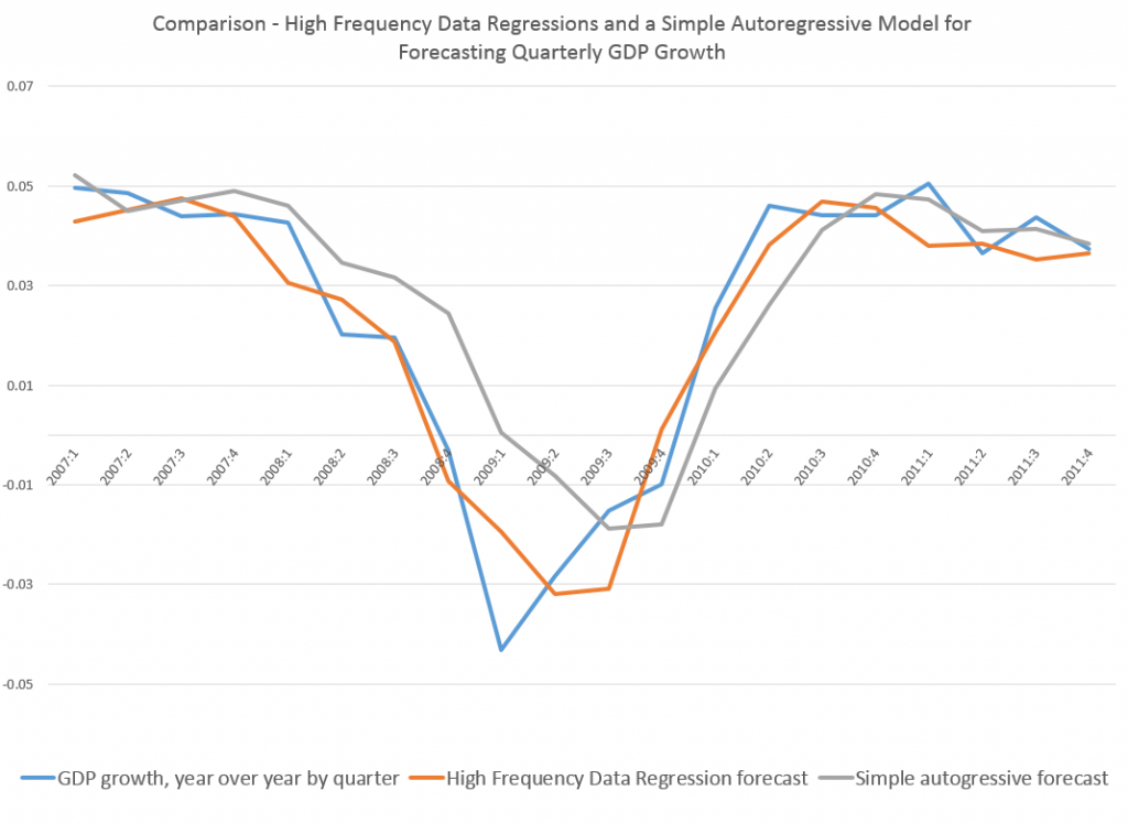
The results are fairly impressive. The regression equation estimated over quarterly and monthly data to the end of 2006 performs much better than a simple first order autocorrelation during the tremendous dip in growth characterizing the Great Recession. In general, even after stabilization of GDP growth in 2010 and 2011, the high frequency data regression produces better out-of-sample forecasts.

Here is a graph comparing the out-of-sample forecast accuracy of the high frequency regression and a simple first order autocorrelation relationship.

MIDAScomp

What’s especially interesting is that the high frequency data regression does a good job of capturing the drop in GDP and the movement at the turning point in 2009 – the depth of the Great Recession.

I throw this chart up as a proof-of-concept. More detailed methods, using a specially-constructed Chicago Fed index, are described in a paper in the Journal of Economic Perspectives.

CO2 Concentrations Spiral Up, Global Temperature Stabilizes – Was Gibst?

Predicting global temperature is challenging. This is not only because climate and weather are complex, but because carbon dioxide (CO2) concentrations continue to skyrocket, while global temperature has stabilized since around 2000.

Changes in Global Mean Temperature

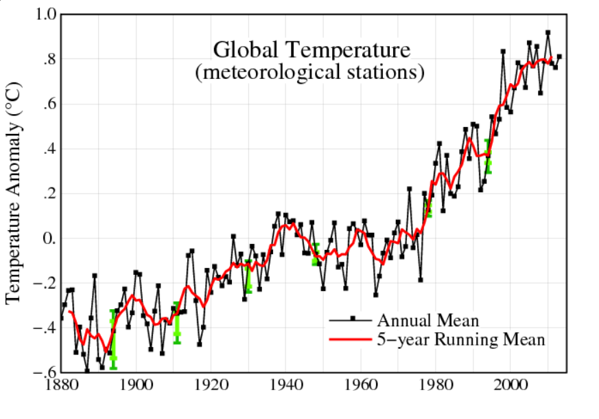
The NASA Goddard Institute for Space Studies maintains extensive and updated charts on global temperature.

globalmeantempdelta

The chart for changes annual mean global temperature is compiled from weather stations from around the planet.

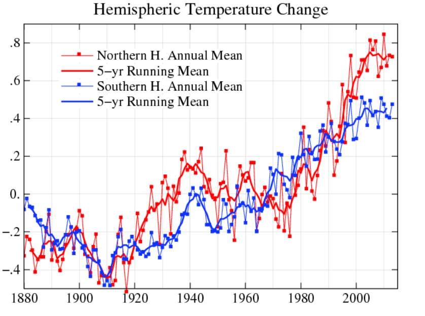
There is also hermispheric variation, with the northern hemisphere showing more increases than the southern hemisphere.

hemi

At the same time, observations of the annual change in mean temperature have stabilized since around 2000, as the five year moving averages show.

Atmospheric Carbon Dioxide Concentrations

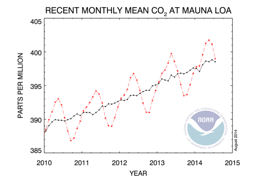
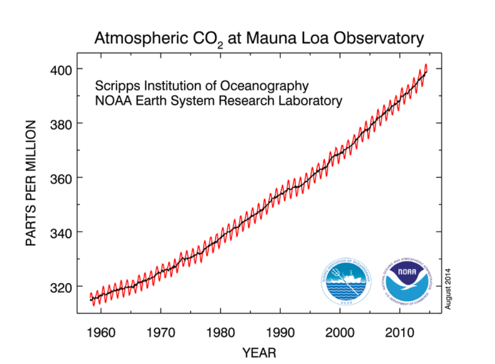
The National Oceanic and Atmospheric Administration (NOAA) maintains measurements of atmospheric carbon dioxide taken in Hawaii at Mauna Loa. These show continual increase since the measurements were first initiated in the late 1950’s.

Here’s a chart showing recent monthly measurements, highlighting the consistent seasonal pattern and strong positive trend since 2010.

Maunaloa1

Here’s all the data. The black line in both charts represents the seasonally corrected trend.

Maunaloa2

A Forecasting Problem

This is a big problem for anyone interested in predicting the future trajectory of climate.

So, according to these measurements on Mauna Loa, carbon dioxide concentrations in the atmosphere have been increasing monotonically (with seasonal variation) since 1958, when measurements first began. Yet global temperatures have not increased on a clear trend since around 2000.

I want to comment in detail sometime on the forecasting controversies that have swirled around these types of measurements and their interpretation, but here let me just suggest the outlines of the problem.

So, it’s clear that the relationship between atmospheric CO2 concentrations and global temperature is not linear, or that there are major intervening variables. Cloud cover may increase with higher temperatures, due to more evaporation. The oceans are still warming, so maybe they are absorbing the additional heat. Perhaps there are other complex feedback processes involved.

However, if my reading of the IPCC literature is correct, these suggestions are still anecdotal, since the big systems models seem quite unable to account for this trajectory of temperature – or at least, recent data appear as outliers.

So there you have it. As noted in earlier posts here, global population is forecast to increase by perhaps one billion by 2030. Global output, even given uncertain impacts of coming recessions, may grow to $150 trillion dollars by 2030. Emissions of greenhouse gases, including but not limited to CO2 also will increase – especially given the paralyzing impacts of the current “pause in global warming” on coordinated policy responses. Deforestation is certainly a problem in this context, although we have not here reviewed the prospects.

One thing to note, however, is that the first two charts presented above trace out changes in global mean temperature by year. The actual level of global mean temperature surged through the 1990’s and remains high. That mean that ice caps are melting, and various processes related to higher temperatures are currently underway.

Recession and Economic Projections

I’ve been studying the April 2014 World Economic Outlook (WEO) of the International Monetary Fund (IMF) with an eye to its longer term projections of GDP.

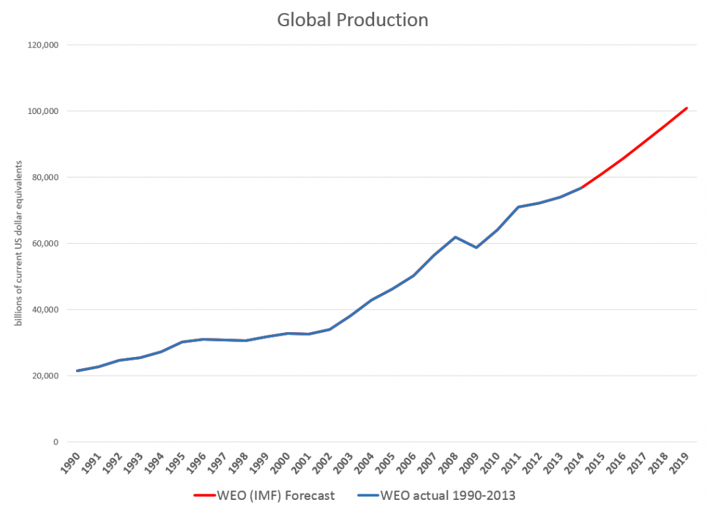
Downloading the WEO database and summing the historic and projected GDP’s suggests this chart.
GlobalGDP

The WEO forecasts go to 2019, almost to our first benchmark date of 2020. Global production is projected to increase from around $76.7 trillion in current US dollar equivalents to just above $100 trillion. An update in July marked the estimated 2014 GDP growth down from 3.7 to 3.4 percent, leaving the 2015 growth estimate at a robust 4 percent.

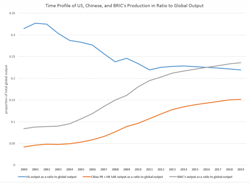
The WEO database is interesting, because it’s country detail allows development of charts, such as this.
gbobalproout

So, based on this country detail on GDP and projections thereof, the BRIC’s (Brazil, Russia, India, and China) will surpass US output, measured in current dollar equivalents, in a couple of years.

In purchasing power parity (PPP) terms, China is currently or will soon pass the US GDP, incidentally. Thus, according to the Big Mac index, a hamburger is 41 percent undervalued in China, compared to the US. So boosting Chinese production 41 percent puts its value greater than US output. However, the global totals would change if you take this approach, and it’s not clear the Chinese proportion would outrank the US yet.

The Impacts of Recession

The method of caging together GDP forecasts to the year 2030, the second benchmark we want to consider in this series of posts, might be based on some type of average GDP growth rate.

However, there is a fundamental issue with this, one I think which may play significantly into the actual numbers we will see in coming years.

Notice, for example, the major “wobble” in the global GDP curve historically around 2008-2009. The Great Recession, in fact, was globally synchronized, although it only caused a slight inflection in Chinese and BRIC growth. Europe and Japan, however, took a major hit, bringing global totals down for those years.

Looking at 2015-2020 and, certainly, 2015-2030, it would be nothing short of miraculous if there were not another globally synchronized recession. Currently, for example, as noted in an earlier post here, the Eurozone, including Germany, moved into zero to negative growth last quarter, and there has been a huge drop in Japanese production. Also, Chinese economic growth is ratcheting down from it atmospheric levels of recent years, facing a massive real estate bubble and debt overhang.

But how to include a potential future recession in economic projections?

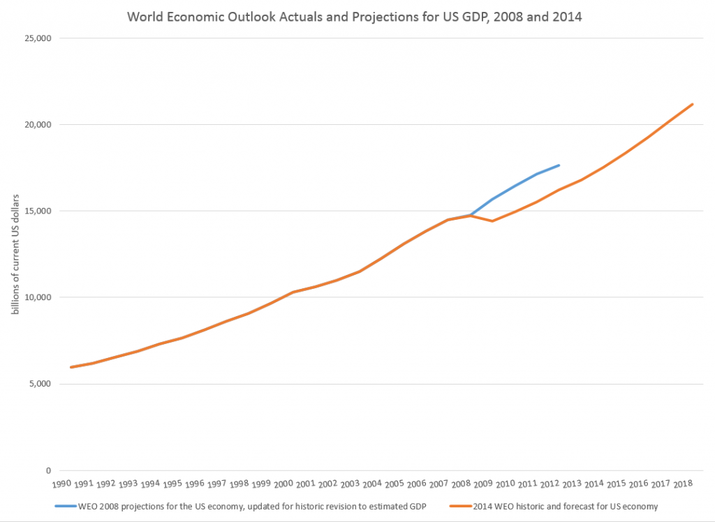
One guide might be to look at how past projections have related to these types of events. Here, for example, is a comparison of the 2008 and 2014 US GDP projections in the WEO’s.
WEOUS

So, according to the IMF, the Great Recession resulted in a continuing loss of US production through until the present.

This corresponds with the concept that, indeed, the GDP time series is, to a large extent, a random walk with drift, as Nelson and Plosser suggested decades ago (triggering a huge controversy over unit roots).

And this chart highlights a meaning for potential GDP. Thus, the capability to produce things did not somehow mysteriously vanish in 2008-2009. Rather, there was no point in throwing up new housing developments in a market that was already massively saturated, Not only that, but the financial sector was unable to perform its usual duties because it was insolvent – holding billions of dollars of apparently worthless collateralized mortgage securities and other financial innovations.

There is a view, however, that over a long period of time some type of mean reversion crops up.

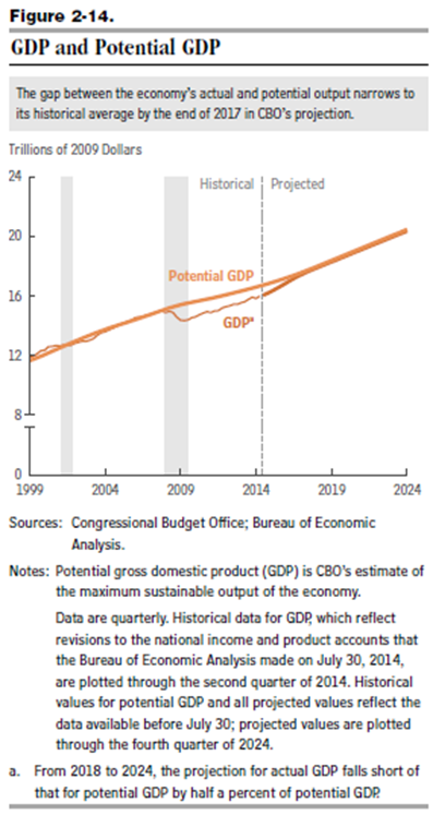
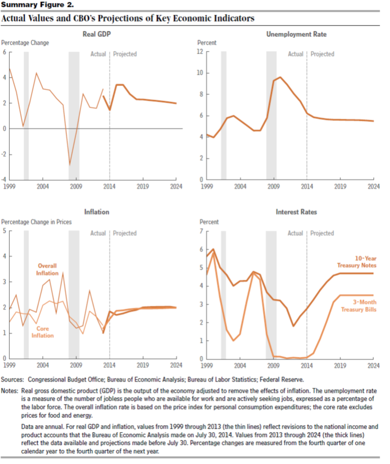
This is exemplified in the 2014 Congressional Budget Office (CBO) projections, as shown in this chart from the underlying detail.
CBOpotentialGDP

This convergence on potential GDP, which somehow is shown in the diagram with a weaker growth rate just after 2008, is based on the following forecasts of underlying drivers, incidentally.
CBOdrivers

So again, despite the choppy historical detail for US real GDP growth in the chart on the upper left, the forecast adopted by the CBO blithely assumes no recession through 2024 as well as increase in US interest rates back to historic levels by 2019.

I think this clearly suggests the Congressional Budget Office is somewhere in la-la land.

But the underlying question still remains.

How would one incorporate the impacts of an event – a recession – which is probably almost a certainty by the end of these forecast horizons, but whose timing is uncertain?

Of course, there are always scenarios, and I think, particularly for budget discussions, it would be good to display one or two of these.

I’m interested in reader suggestions on this.

Video Friday – The Present Can Influence the Past?

In forecasting, the common assumption is that the present influences the future, but the opposite does not occur.

Oh to be sure, one develops expectations and, yes, predictions which may influence present actions. But these are not realized, but projected. What actually occurs tomorrow, however, is not usually considered to directly influence what transpires today, particularly chance events. Thus, if Roger flips a coin tomorrow and it comes up heads, that is not supposed to have any material effect on physical processes occurring today.

But this turns out to happen at the level of quantum reality – in other words, at a more fundamental level of physical reality, as the quantum eraser experiment proves.

OK, it is a good idea to begin with the classic double slit experiment, as a lead-in. Here are two videos, one with a comic strip professor, and the second with Professor Brian Greene of Columbia University and several of his collegues.


So you immediately get into what I would call metaphysics – issues of whether consciousness can impinge on what is being observed, thus changing it.

Again, Professor Brian Greene on the double slit experiment, another narrative.

 OK, so then there is the “quantum eraser.”

 I’m still thinking about this. It’s profound, experimental metaphysics. Time is not what we think it is, just as space is not what it seems.

Quantum entanglement, incidentally, is what Einstein called “spooky action at a distance.”

Random Cycles

In 1927, the Russian statistician Eugen Slutsky wrote a classic article called ‘The summation of random causes as the source of cyclic processes,’ a short summary of which is provided by Barnett

If the variables that were taken to represent business cycles were moving averages of past determining quantities that were not serially correlated – either real-world moving averages or artificially generated moving averages – then the variables of interest would become serially correlated, and this process would produce a periodicity approaching that of sine waves

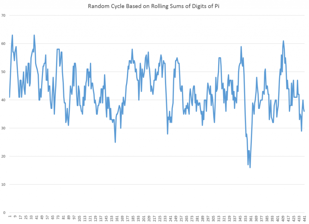
It’s possible to illustrate this phenomena with rolling sums of the digits of pi (π). The following chart illustrates the wave-like result of charting rolling sums of ten consecutive digits of pi.

picycle

So to be explicit, I downloaded the first 450 digits of pi, took them apart, and then graphed the first 440 rolling sums.

The wave-like pattern Illustrates a random cycle.

Forecasting Random Cycles

If we consider this as a time series, each element xk is the following sum,

xk = dk+dk-1+..+dk-10

where dj is the jth digit in the decimal expansion of pi to the right of the initial value of 3.

Now, apparently, it is not proven that the digits of pi are truly random, although one can show that, so far as we can compute, these digits are described by a uniform distribution.

As far as we know, the probability that the next digit will be any digit from 0 to 9 is 1/10=0.1

So as one moves through the digits of pi, generating rolling sums, each new sum means the addition of a new digit, which is unknown and can only be predicted up to its probability. And, at the same time, a digit at the beginning of the preceding sum drops away in the new sum.

Note also that we can always deduce what the series of original digits is, given a series of these rolling sums up to some point.

So the issue is whether the new digit added to the next sum is greater than, equal to, or less than the leading digit of the current sum – which is where we now stand in this sort of analysis. This determines whether the next rolling sum will be greater than, equal to, or less than the current sum.

Here’s where the forecasts can be produced. If the rolling sum is large enough, approaching or equal to 90, there is a high probability that the next rolling sum will be lower, leading to this wave-like pattern. Conversely, if the rolling sum is near zero, the chances are the subsequent sum will be larger. And all this arm-waving can be complemented by exact probabilistic calculations.

Some Ultimate Thoughts

It’s interesting we are really dealing here with a random cycle. That’s proven by the fact that, at any time, the series could go flat-line or trace out some other kind of weird movement.

Thus, the quasi-periodic aspect can be violated for as many periods as you might choose, if one arrives at a run of the same digit in the expansion of pi.

This reminds me of something George Gamow wrote in one of his popular books, where he discusses thermodynamics and the random movement of atoms and molecules in the air of a room. Gamow observes it is entirely possible all the air by chance will congregate in one corner, leaving a vacuum elsewhere. Of course, this is highly improbable.

The only difference would be that there are a finite number of atoms and molecules in the air of any room, but, presumably, an infinite number of digits in the expansion of pi.

The morale of the story is, in any case, to be cautious in imposing a fixed cycle on this type of series.

Selecting Predictors – the Specification Problem

I find toy examples helpful in exploratory work.

So here is a toy example showing the pitfalls of forward selection of regression variables, in the presence of correlation between predictors. In other words, this is an example of the specification problem.

Suppose the true specification or regression is –

y = 20x1-11x2+10x3

and the observations on x2 and x3 in the available data are correlated.

To produce examples of this system, I create columns of random numbers in which the second and third columns are correlated with a correlation coefficient of around 0.6. I also add a random error term with zero mean and constant variance of 10. Then, after generating the data and the error terms, I apply the coefficients indicated above and estimate values for the dependent variable y.

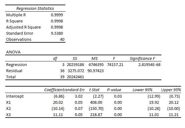
Then, specifying all three variables,  x1, x2, and x3, I estimate regressions which characteristically have coefficient values not far from the (20,-11, 10), such as,

spregThis, of course, is a regression output from Microsoft Excel, where I developed this simple Monte Carlo simulation which has 40 “observations.”

If you were lucky enough to estimate this regression initially, you well might stop and not bother about dropping variables to estimate other potentially competing models.

However, if you start with fewer variables, you encounter a significant difficulty.

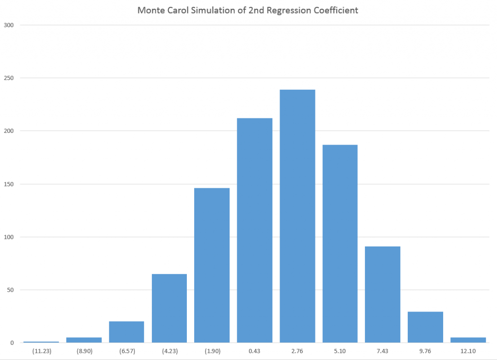
Here is the distribution of x2 in repeated estimates of a regression with explanatory variables x1 and x2 –

coeff2

As you can see, the various estimates of the value of this coefficient, whose actual or true value is -11, are wide of the mark. In fact, none of the 1000 estimates in this simulation proved to be statistically significant at standard levels.

Using some flavors of forward regression, therefore, you well might decide to drop x2 in the specification and try including x3.

But you would have the same type of problem in that case, too, since x2 and x3 are correlated.

I sometimes hear people appealing to stability arguments in the face of the specification problem. In other words, they strive to find a stable set of core predictors, believing that if they can do this, they will have controlled as effectively as they can for this problem of omitted variables which are correlated with other variables that are included in the specification.

Top Forecasting Institutions and Researchers According to IDEAS!

Here is a real goldmine of research on forecasting.

IDEAS! is a RePEc service hosted by the Research Division of the Federal Reserve Bank of St. Louis.

This website compiles rankings on authors who have registered with the RePEc Author Service, institutions listed on EDIRC, bibliographic data collected by RePEc, citation analysis performed by CitEc and popularity data compiled by LogEc – under the category of forecasting.

Here is a list of the top fifteen of the top 10% institutions in the field of forecasting, according to IDEAS!. The institutions are scored based on a weighted sum of all authors affiliated with the respective institutions (click to enlarge).

top15ForecastingSchool

The Economics Department of the University of Wisconsin, the #1 institution, lists 36 researchers who claim affiliation and whose papers are listed under the category forecasting in IDEAS!.

The same IDEAS! Webpage also lists the top 10% authors in the field of forecasting. I extract the top 20 of this list here below. If you click through on an author, you can see their list of publications, many of which often are available as PDF downloads.

IDEASauthors20

This is a good place to start in updating your knowledge and understanding of current thinking and contextual issues relating to forecasting.

The Applied Perspective

For an applied forecasting perspective, there is Bloomberg with this fairly recent video on several top economic forecasters providing services to business and investors.

I believe Bloomberg will release extensive, updated lists of top forecasters by country, based on a two year perspective, in a few weeks.