Tag Archives: Big Data

Big Data, data mining, data science, kernel ridge regression

Kernel Ridge Regression – A Toy Example

March 1, 2014 Clive Jones

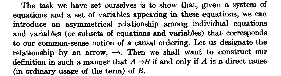
Kernel ridge regression (KRR) is a promising technique in forecasting and other applications, when there are “fat” databases. It’s intrinsically “Big Data” and can accommodate nonlinearity, in addition to many predictors.

Kernel ridge regression, however, is shrouded in mathematical complexity. While this is certainly not window-dressing, it can obscure the fact that the method is no different from ordinary ridge regression on transformations of regressors, except for an algebraic trick to improve computational efficiency.

This post develops a spreadsheet example illustrating this key point – kernel ridge regression is no different from ordinary ridge regression…except for an algebraic trick.

Background

Most applications of KRR have been in the area of machine learning, especially optical character recognition.

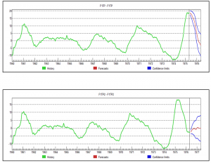
To date, the primary forecasting application involves a well-known “fat” macroeconomic database. Using this data, researchers from the Tinbergen Institute and Erasmus University develop KRR models which outperform principal component regressions in out-of-sample forecasts of variables, such as real industrial production and employment.

You might want to tab and review several white papers on applying KRR to business/economic forecasting, including,

Nonlinear Forecasting with Many Predictors using Kernel Ridge Regression

Modelling Issues in Kernel Ridge Regression

Model Selection in Kernel Ridge Regression

This research holds out great promise for KRR, concluding, in one of these selections that,

The empirical application to forecasting four key U.S. macroeconomic variables — production, income, sales, and employment — shows that kernel-based methods are often preferable to, and always competitive with, well-established autoregressive and principal-components-based methods. Kernel techniques also outperform previously proposed extensions of the standard PC-based approach to accommodate nonlinearity.

Calculating a Ridge Regression (and Kernel Ridge Regression)

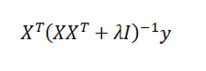
Recall the formula for ridge regression,

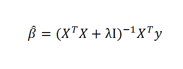
Here, X is the data matrix, X^Tis the transpose of X, λ is the conditioning factor, I is the identify matrix, and y is a vector of values of the dependent or target variable. The “beta-hats” are estimated β’s or coefficient values in the conventional linear regression equation,

y = β₁x₁+ β₂x₂+… β_Nx_N

The conditioning factor λ is determined by cross-validation or holdout samples (see Hal Varian’s discussion of this in his recent paper).

Just for the record, ridge regression is a data regularization method which works wonders when there are glitches – such as multicollinearity – which explode the variance of estimated coefficients.

Ridge regression, and kernel ridge regression, also can handle the situation where there are more predictors or explanatory variables than cases or observations.

A Specialized Dataset

Now let us consider ridge regression with the following specialized dataset.

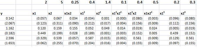
By construction, the equation,

y = 2x₁ + 5x₂+0.25x₁x₂+0.5x₁²+1.5x₂²+0.5x₁x₂²+0.4x₁²x₂+0.2x₁³+0.3x₂³

generates the six values of y from the sums of ten terms in x1 and x2, their powers, and cross-products.

Although we really only have two explanatory variables, x₁ and x_2,the equation, as a sum of 10 terms, can be considered to be constructed out of ten, rather than two, variables.

However, adopting this convenience, it means we have more explanatory variables (10) than observations on the dependent variable (6).

Thus, it will be impossible to estimate the beta’s by OLS.

Of course, we can develop estimates of the values of the coefficients of the true relationship between y and the data on the explanatory variables with ridge regression.

Then, we will find that we can map all ten of these apparent variables in the equation onto a kernel of two variables, simplifying the matrix computations in a fundamental way, using this so-called algebraic trick.

The ordinary ridge regression data matrix X is 6 rows by 10 columns, since there are six observations or cases and ten explanatory variables. Thus, the transpose X^T is a 10 by 6 matrix. Accordingly, the product X^TX is a 10 by 10 matrix, resulting in a 10 by 10 inverse matrix after the conditioning factor and identity matrix is added in to X^TX.

In fact, the matrix equation for ridge regression can be calculated within a spreadsheet using the Excel functions mmult(.,) and minverse() and the transpose operation from Copy. The conditioning factor λ can be determined by trial and error, or by writing a Visual Basic algorithm to explore the mean square error of parameter values associated with different values λ.

The ridge regression formula above, therefore, gives us estimates for ten beta-hats, as indicated in the following chart, using a λ or conditioning coefficient of .005.

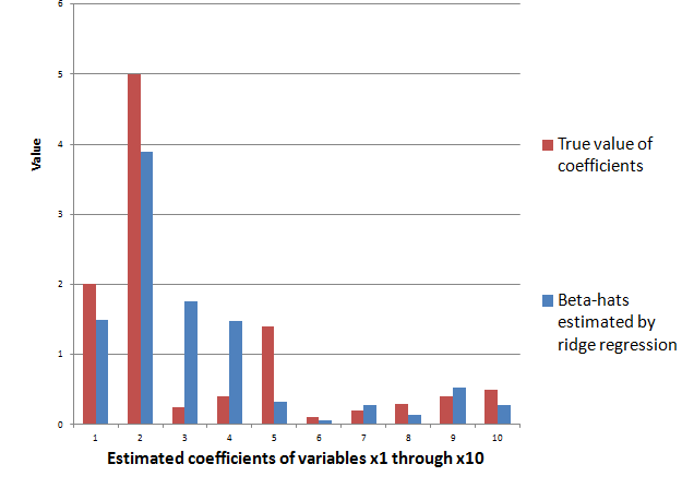
The red bars indicate the true coefficient values, and the blue bars are the beta-hats estimated by the ridge regression formula.

As you can see, ridge regression “gets in the ballpark” in terms of the true values of the coefficients of this linear expression. However, with only 6 observations, the estimate is highly approximate.

The Kernel Trick

Now with suitable pre- and post-multiplications and resorting, it is possible to switch things around to another matrix formula,

Exterkate et al show the matrix algebra in a section of their “Nonlinear..” white paper using somewhat different symbolism.

Key point – the matrix formula listed just above involves inverting a smaller matrix, than the original formula – in our example, a 6 by 6, rather than a 10 by 10 matrix.

The following Table shows the beta-hats estimated by these two formulas are similar and compares them with the “true” values of the coefficients.

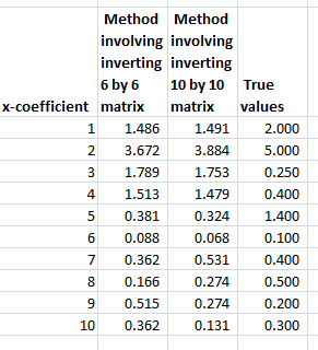
Differences in the estimates by these formally identical formulas relate strictly to issues at the level of numerical analysis and computation.

Kernels

Notice that the ten variables could correspond to a Taylor expansion which might be used to estimate the value of a nonlinear function. This is a key fact and illustrates the concept of a “kernel”.

Thus, designating K = XX^T_,we find that the elements of K can be obtained without going through the indicated multiplication of these two matrices. This is because K is a polynomial kernel.

There is a great deal more that can be said about this example and the technique in general. Two big areas are (a) arriving at the estimate of the conditioning factor λ and (b) discussing the range of possible kernels that can be used, what makes a kernel a kernel, how to generate kernels from existing kernels, where Hilbert spaces come into the picture, and so forth.

But hopefully this simple example can point the way.

For additional insight and the source for the headline Homer Simpson graphic, see The Kernel Trick.

analytical software, Big Data, Chinese economy, data mining, data science, developing country forecast

Links – February 28

February 28, 2014 Clive Jones

Data Science and Predictive Analytics

Data Scientists Predict Oscar® Winners Again; Social Media May Love Leo, But Data Says “No”

..the data shows that Matthew McConaughey will win best actor for his role in the movie Dallas Buyers Guide; Alfonso Cuaron will win best director for the movie Gravity; and 12 Months a Slave will win the coveted prize for best picture – which is the closest among all the races. The awards will not be a clean sweep for any particular picture, although the other award winners are expected to be Jared Leto for best supporting actor in Dallas Buyers Club; Cate Blanchet for best actress in Blue Jasmine; and Lupita Nyong’o for best supporting actress in 12 Years a Slave.

10 Most Influential Analytics Leaders in India

Pankaj Kulshreshtha – Business Leader, Analytics & Research at Genpact

Rohit Tandon – Vice President, Strategy WW Head of HP Global Analytics

Sameer Dhanrajani – Business Leader, Cognizant Analytics

Srikanth Velamakanni – Co founder and Chief Executive Officer at Fractal Analytics

Pankaj Rai – Director, Global Analytics at Dell

Amit Khanna – Partner at KPMG

Ashish Singru – Director eBay India Analytics Center

Arnab Chakraborty – Managing Director, Analytics at Accenture Consulting

Anil Kaul – CEO and Co-founder at Absolutdata

Dr. N.R.Srinivasa Raghavan, Senior Vice President & Head of Analytics at Reliance Industries Limited

Interview with Jörg Kienitz, co-author with Daniel Wetterau of Financial Modelling: Theory, Implementation and Practice with MATLAB Source

JB: Why MATLAB? Was there a reason for choosing it in this context?

JK: Our attitude was that it was a nice environment for developing models because you do not have to concentrate on the side issues. For instance, if you want to calibrate a model you can really concentrate on implementing the model without having to think about the algorithms doing the optimisation for example. MATLAB offers a lot of optimisation routines which are really reliable and which are fast, which are tested and used by thousands of people in the industry. We thought it was a good idea to use standardised mathematical software, a programming language where all the mathematical functions like optimisation, like Fourier transform, random number generator and so on, are very reliable and robust. That way we could concentrate on the algorithms which are necessary to implement models, and not have to worry about a programming a random number generator or such stuff. That was the main idea, to work on a strong ground and build our house on a really nice foundation. So that was the idea of choosing MATLAB.

Knowledge-based programming: Wolfram releases first demo of new language, 30 years in the making

Economy

Credit Card Debt Threatens Turkey’s Economy – kind of like the subprime mortgage scene in the US before 2008.

..Standard & Poor’s warned in a report last week that the boom in consumer credit had become a serious risk for Turkish lenders. Slowing economic growth, political turmoil and increasing reluctance by foreign investors to provide financing “are prompting a deterioration in the operating environment for Turkish banks,”

A shadow banking map from the New York Fed. Go here and zoom in for detail.

China Sees Expansion Outweighing Yuan, Shadow Bank Risk

China’s Finance Minister Lou Jiwei played down yuan declines and the risks from shadow banking as central bank Governor Zhou Xiaochuan signaled that the nation’s economy can sustain growth of between 7 percent and 8 percent.

Outer Space

715 New Planets Found (You Read That Number Right)

Speaks for itself. That’s a lot of new planets. One of the older discoveries – Tau Boötis b – has been shown to have water vapor in its atmosphere.

Hillary, ‘The Family,’ and Uganda’s Anti-Gay Christian Mafia

I heard about this at the SunDance film gathering in 2013. Apparently, there are links between US and Ugandan groups in promulgating this horrific law.

An Astronaut’s View of the North Korean Electricity Black Hole

Big Data, causal networks, Medical data analytics, predictive analytics

Using Math to Cure Cancer

February 27, 2014 Clive Jones

There are a couple of takes on this.

One is like “big data and data analytics supplanting doctors.”

So Dr. Cary Oberije certainly knows how to gain popularity with conventional-minded doctors.

In Mathematical Models Out-Perform Doctors in Predicting Cancer Patients’ Responses to Treatment she reports on research showing predictive models are better than doctors at predicting the outcomes and responses of lung cancer patients to treatment… “The number of treatment options available for lung cancer patients are increasing, as well as the amount of information available to the individual patient. It is evident that this will complicate the task of the doctor in the future,” said the presenter, Dr Cary Oberije, a postdoctoral researcher at the MAASTRO Clinic, Maastricht University Medical Center, Maastricht, The Netherlands. “If models based on patient, tumor and treatment characteristics already out-perform the doctors, then it is unethical to make treatment decisions based solely on the doctors’ opinions. We believe models should be implemented in clinical practice to guide decisions.”

Dr Oberije says,

“Correct prediction of outcomes is important for several reasons… First, it offers the possibility to discuss treatment options with patients. If survival chances are very low, some patients might opt for a less aggressive treatment with fewer side-effects and better quality of life. Second, it could be used to assess which patients are eligible for a specific clinical trial. Third, correct predictions make it possible to improve and optimise the treatment. Currently, treatment guidelines are applied to the whole lung cancer population, but we know that some patients are cured while others are not and some patients suffer from severe side-effects while others don’t. We know that there are many factors that play a role in the prognosis of patients and prediction models can combine them all.”

At present, prediction models are not used as widely as they could be by doctors…. some models lack clinical credibility; others have not yet been tested; the models need to be available and easy to use by doctors; and many doctors still think that seeing a patient gives them information that cannot be captured in a model.

Dr. Oberije asserts, Our study shows that it is very unlikely that a doctor can outperform a model.

Along the same lines, mathematical models also have been deployed to predict erectile dysfunction after prostate cancer.

I think Dr. Oberije is probably right that physicians could do well to avail themselves of broader medical databases – on prostate conditions, for example – rather than sort of shooting from the hip with each patient.

The other approach is “teamwork between physicians, data and other analysts should be the goal.”

So it’s with interest I note the Moffit Cancer Center in Tampa Florida espouses a teamwork concept in cancer treatment with new targeted molecular therapies.

The IMO program’s approach is to develop mathematical models and computer simulations to link data that is obtained in a laboratory and the clinic. The models can provide insight into which drugs will or will not work in a clinical setting, and how to design more effective drug administration schedules, especially for drug combinations. The investigators collaborate with experts in the fields of biology, mathematics, computer science, imaging, and clinical science.

“Limited penetration may be one of the main causes that drugs that showed good therapeutic effect in laboratory experiments fail in clinical trials,” explained Rejniak. “Mathematical modeling can help us understand which tumor, or drug-related factors, hinder the drug penetration process, and how to overcome these obstacles.”

A similar story cropped up in in the Boston Globe – Harvard researchers use math to find smarter ways to defeat cancer

Now, a new study authored by an unusual combination of Harvard mathematicians and oncologists from leading cancer centers uses modeling to predict how tumors mutate to foil the onslaught of targeted drugs. The study suggests that administering targeted medications one at a time may actually insure that the disease will not be cured. Instead, the study suggests that drugs should be given in combination.

header picture: http://www.en.utexas.edu/Classes/Bremen/e316k/316kprivate/scans/hysteria.html

ARIMA models, Big Data, macroeconomic forecasting, principal component models and forecasts

Forecasting and Data Analysis – Principal Component Regression

February 26, 2014 Clive Jones

I get excited that principal components offer one solution to the problem of the curse of dimensionality – having fewer observations on the target variable to be predicted, than there are potential drivers or explanatory variables.

It seems we may have to revise the idea that simpler models typically outperform more complex models.

Principal component (PC) regression has seen a renaissance since 2000, in part because of the work of James Stock and Mark Watson (see also) and Bai in macroeconomic forecasting (and also because of applications in image processing and text recognition).

Let me offer some PC basics and explore an example of PC regression and forecasting in the context of macroeconomics with a famous database.

Dynamic Factor Models in Macroeconomics

Stock and Watson have a white paper, updated several times, in PDF format at this link

stock watson generalized shrinkage June _2012.pdf

They write in the June 2012 update,

We find that, for most macroeconomic time series, among linear estimators the DFM forecasts make efficient use of the information in the many predictors by using only a small number of estimated factors. These series include measures of real economic activity and some other central macroeconomic series, including some interest rates and monetary variables. For these series, the shrinkage methods with estimated parameters fail to provide mean squared error improvements over the DFM. For a small number of series, the shrinkage forecasts improve upon DFM forecasts, at least at some horizons and by some measures, and for these few series, the DFM might not be an adequate approximation. Finally, none of the methods considered here help much for series that are notoriously difficult to forecast, such as exchange rates, stock prices, or price inflation.

Here DFM refers to dynamic factor models, essentially principal components models which utilize PC’s for lagged data.

What’s a Principal Component?

Essentially, you can take any bundle of data and compute the principal components. If you mean-center and (in most cases) standardize the data, the principal components divide up the variance of this data, based on the size of their associated eigenvalues. The associated eigenvectors can be used to transform the data into an equivalent and same size set of orthogonal vectors. Really, the principal components operate to change the basis of the data, transforming it into an equivalent representation, but one in which all the variables have zero correlation with each other.

The Wikipaedia article on principal components is useful, but there is no getting around the fact that principal components can only really be understood with matrix algebra.

Often you see a diagram, such as the one below, showing a cloud of points distributed around a line passing through the origin of a coordinate system, but at an acute angle to those coordinates.

This illustrates dimensionality reduction with principal components. If we express all these points in terms of this rotated set of coordinates, one of these coordinates – the signal – captures most of the variation in the data. Projections of the datapoints onto the second principal component, therefore, account for much less variance.

Principal component regression characteristically specifies only the first few principal components in the regression equation, knowing that, typically, these explain the largest portion of the variance in the data.

It’s also noteworthy that some researchers are talking about “targeted” principal components. So the first few principal components account for the largest, the next largest, and so on amount of variance in the data. However, the “data” in this context does not include the information we have on the target variable. Targeted principal components therefore involves first developing the simple correlations between the target variable and all the potential predictors, then ordering these potential predictors from highest to lowest correlation. Then, by one means or another, you establish a cutoff, below which you exclude weak potential predictors from the data matrix you use to compute the principal components. Interesting approach which makes sense. Testing it with a variety of examples seems in order.

PC Regression and Forecasting – A Macroeconomics Example

I downloaded a trial copy of XLSTAT – an Excel add-in with a well-developed set of principal component procedures. In the past, I’ve used SPSS and SAS on corporate networked systems. Now I am using Matlab and GAUSS for this purpose.

The problem is what does it mean to have a time series of principal components? Over the years, there have been relevant discussions – Jolliffe’s key work, for example, and more recent papers.

The problem with time series, apart from the temporal interdependencies, is that you always are calculating the PC’s over different data, as more data comes in. What does this do to the PC’s or factor scores? Do they evolve gradually? Can you utilize the factor scores from a smaller dataset to predict subsequent values of factor scores estimated over an augmented dataset?

Based on a large macroeconomic dataset I downloaded from Mark Watson’s page, I think the answer can be a qualified “yes” to several of these questions. The Mark Watson dataset contains monthly observations on 106 macroeconomic variables for the period 1950 to 2006.

For the variables not bounded within a band, I calculated year-over-year (yoy) growth rates for each monthly observation. Then, I took first differences again over 12 months. These transformations eliminated trends, which mess up the PC computations (basically, if you calculate PC’s with a set of increasing variables, the first PC will represent a common growth factor, and is almost useless for modeling purposes.) The result of my calculations was to center each series at nearly zero, and to make the variability of each series comparable – so I did not standardize.

Anyway, using XLSTAT and Forecast Pro – I find that the factor scores

(a) Evolve slowly as you add more data.

(b) Factor scores for smaller datasets provide insight into subsequent factor scores one to several months ahead.

(c) Amazingly, turning points of the first principal component, which I have studied fairly intensively, are remarkably predictable.

So what are we looking at here (click to enlarge)?

Well, the top chart is the factor score for the first PC, estimated over data to May 1975, with a forecast indicated by the red line at the right of the graph. This forecast produces values which are very close to the factor score values for data estimated to May 1976 – where both datasets begin in 1960. Not only that, but we have here an example of prediction of a turning point bigtime.

Of course this is the magic of Box-Jenkins, since, this factor score series is best estimated, according to Forecast Pro, with an ARIMA model.

I’m encouraged by this exercise to think that it may be possible to go beyond the lagged variable specification in many of these DFM’s to a contemporaneous specification, where the target variable forecasts are based on extrapolations of the relevant PC’s.

In any case, for applied business modeling, if we got something like a medical device new order series (suitably processed data) linked with these macro factor scores, it could be interesting – and we might get something that is not accessible with ordinary methods of exponential smoothing.

Underlying Theory of PC’s

Finally, I don’t think it is possible to do much better than to watch Andrew Ng at Stanford in Lectures 14 and 15. I recommend skipping to 17:09 – seventeen minutes and nine seconds – into Lecture 14, where Ng begins the exposition of principal components. He winds up this Lecture with a fascinating illustration of high dimensionality principal component analysis applied to recognizing or categorizing faces in photographs at the end of this lecture. Lecture 15 also is very useful – especially as it highlights the role of the Singular Value Decomposition (SVD) in actually calculating principal components.

Lecture 14

http://www.youtube.com/watch?v=ey2PE5xi9-A

Lecture 15

http://www.youtube.com/watch?v=QGd06MTRMHs

Bayesian networks, causal discovery, causal networks

Causal and Bayesian Networks

February 18, 2014 Clive Jones

In his Nobel Acceptance Lecture, Sir C.J.W. Granger mentions that he did not realize people had so many conceptions of causality, nor that his proposed test would be so controversial – resulting in its being confined to a special category “Granger Causality.’

That’s an astute observation – people harbor many conceptions and shades of meaning for the idea of causality. It’s in this regard that renewed efforts recently – motivated by machine learning – to operationalize the idea of causality, linking it with both directed graphs and equation systems, is nothing less than heroic.

However, despite the confusion engendered by quantum theory and perhaps other “new science,” the identification of “cause” can be materially important in the real world. For example, if you are diagnosed with metastatic cancer, it is important for doctors to discover where in the body the cancer originated – in the lungs, in the breast, and so forth. This can be challenging, because cancer mutates, but making this identification can be crucial for selecting chemotherapy agents. In general, medicine is full of problems of identifying causal nexus, cause and effect.

In economics, Herbert Simon, also a Nobel Prize recipient, actively promoted causal analysis and its representation in graphs and equations. In Causal Ordering and Identifiability, Simon writes,

For example, we cannot reverse the causal chain poor growing weather → small wheat crops → increase in price of wheat by an attribution increase in price of wheat → poor growing weather.

Simon then proposes that the weather to price causal system might be represented by a series of linear, simultaneous equations, as follows:

This example can be solved recursively, first by solving for x1, then by using this value of x1 to solve for x2, and then using the so-obtained values of x1 and x2 to solve for x3. So the system is self-contained, and Simon discusses other conditions. Probably the most important is assymmetry and the direct relationship between variables.

Readers interested in the milestones in this discourse, leading to the present, need to be aware of Pearl’s seminal 1998 article, which begins,

It is an embarrassing but inescapable fact that probability theory, the official mathematical language of many empirical sciences, does not permit us to express sentences such as “”Mud does not cause rain”; all we can say is that the two events are mutually correlated, or dependent – meaning that if we find one, we can expect to encounter the other.”

Positive Impacts of Machine Learning

So far as I can tell, the efforts of Simon and even perhaps Pearl would have been lost in endless and confusing controversy, were it not for the emergence of machine learning as a distinct specialization

A nice, more recent discussion of causality, graphs, and equations is Denver Dash’s A Note on the Correctness of the Causal Ordering Algorithm. Dash links equations with directed graphs, as in the following example.

Dash shows that Simon’s causal ordering algorithm (COA) to match equations to a cluster graph is consistent with more recent methods of constructing directed causal graphs from the same equation set.

My reading suggests a direct line of development, involving attention to the vertices and nodes of directed acyclic graphs (DAG’s) – or graphs without any backward connections or loops – and evolution to Bayesian networks – which are directed graphs with associated probabilities.

Here is are two examples of Bayesian networks.

First, another contribution from Dash and others

So clearly Bayesian networks are closely akin to expert systems, combining elements of causal reasoning, directed graphs, and conditional probabilities.

The scale of Bayesian networks can be much larger, or societal-wide, as this example from Using Influence Nets in Financial Informatics: A Case Study of Pakistan.

The development of machine systems capable of responding to their environment – robots, for example – are a driver of this work currently. This leads to the distinction between identifying causal relations by observation or from existing data, and from intervention, action, or manipulation. Uncovering mechanisms by actively energizing nodes in a directed graph, one-by-one, is, in some sense, an ideal approach. However, there are clearly circumstances – again medical research provides excellent examples – where full-scale experimentation is simply not possible or allowable.

At some point, combinatorial analysis is almost always involved in developing accurate causal networks, and certainly in developing Bayesian networks. But this means that full implementation of these methods must stay confined to smaller systems, cut corners in various ways, or wait for development (one hopes) of quantum computers.

Note: header cartoon from http://xkcd.com/552/

alternative technology, Big Data, Chinese economy, technology forecasting

Links – February 14

February 14, 2014 Clive Jones

Global Economy

Yellen Says Recovery in Labor Market Far From Complete – Highlights of Fed Chair Yellen’s recent testimony before the House Financial Services Committee. Message – continuity, steady as she goes unless a there is a major change in outlook.

OECD admits overstating growth forecasts amid eurozone crisis and global crash The Paris-based organisation said it repeatedly overestimated growth prospects for countries around the world between 2007 and 2012. The OECD revised down forecasts at the onset of the financial crisis, but by an insufficient degree, it said….

The biggest forecasting errors were made when looking at the prospects for the next year, rather than the current year.

10 Books for Understanding China’s Economy

Information Technology (IT)

Predicting Crowd Behavior with Big Public Data

Internet startups

Alternative Technology

World’s Largest Rooftop Farm Documents Incredible Growth High Above Brooklyn

bagging, boosting, classification models, ensemble forecasts, random subspace ensemble methods

Random Subspace Ensemble Methods (Random Forest™ algorithm)

February 12, 2014 Clive Jones

As a term, random forests apparently is trademarked, which is, in a way, a shame because it is so evocative – random forests, for example, are comprised of a large number of different decision or regression trees, and so forth.

Whatever the name we use, however, the Random Forest™ algorithm is a powerful technique. Random subspace ensemble methods form the basis for several real world applications, such as Microsoft’s Kinect, facial recognition programs in cell phone and other digital cameras, and figure importantly in many Kaggle competitions, according to Jeremy Howard, formerly Kaggle Chief Scientist.

I assemble here a Howard talk from 2011 called “Getting In Shape For The Sport Of Data Science” and instructional videos from a data science course at the University of British Columbia (UBC). Watching these involves a time commitment, but it’s possible to let certain parts roll and then to skip ahead. Be sure and catch the last part of Howard’s talk, since he’s good at explaining random subspace ensemble methods, aka random forests.

It certainly helps me get up to speed to watch something, as opposed to reading papers on a fairly unfamiliar combination of set theory and statistics.

By way of introduction, the first step is to consider a decision tree. One of the UBC videos notes that decision trees faded from popularity some decades ago, but have come back with the emergence of ensemble methods.

So a decision tree is a graph which summarizes the classification of multi-dimensional points in some space, usually based on creating rectangular areas with reference to the coordinates. The videos make this clearer.

So this is nice, but decision trees of this sort tend to over-fit; they may not generalize very well. There are methods of “pruning” or simplification which can help generalization, but another tactic is to utilize ensemble methods. In other words, develop a bunch of decision trees classifying some set of multi-attribute items.

Random forests simply build such decision trees with a randomly selected group of attributes, subsets of the total attributes defining the items which need to be classified.

The idea is to build enough of these weak predictors and then average to arrive at a modal or “majority rule” classification.

Here’s the Howard talk.

Then, there is an introductory UBC video on decision trees

This video goes into detail on the method of constructing random forests.

Then the talk on random subspace ensemble applications.

asset bubbles, Big Data, Chinese economy, data mining, data science, developing country forecast, forecasting asset bubbles, global business forecasts, IBM Watson, machine learning, macroeconomic forecasting, predictive analytics

Links – February 1, 2014

February 1, 2014 Clive Jones

IT and Big Data

Kayak and Big Data Kayak is adding prediction of prices of flights over the coming 7 days to its meta search engine for the travel industry.

China’s Lenovo steps into ring against Samsung with Motorola deal Lenovo Group, the Chinese technology company that earns about 80 percent of its revenue from personal computers, is betting it can also be a challenger to Samsung Electronics Co Ltd and Apple Inc in the smartphone market.

5 Things To Know About Cognitive Systems and IBM Watson Rob High video on Watson at http://www.redbooks.ibm.com/redbooks.nsf/pages/watson?Open. Valuable to review. Watson is probably different than you think. Deep natural language processing.

Playing Computer Games and Winning with Artificial Intelligence (Deep Learning) Pesents the first deep learning model to successfully learn control policies directly from high-dimensional sensory input using reinforcement learning. The model is a convolutional neural network, trained with a variant of Q-learning, whose input is raw pixels and whose output is a value function estimating future rewards… [applies] method to seven Atari 2600 games from the Arcade Learning Environment, with no adjustment of the architecture or learning algorithm…outperforms all previous approaches on six of the games and surpasses a human expert on three of them.

Global Economy

China factory output points to Q1 lull Chinese manufacturing activity slipped to its lowest level in six months, with indications of slowing growth for the quarter to come in the world’s second-largest economy.

Japan inflation rises to a 5 year high, output rebounds Japan’s core consumer inflation rose at the fastest pace in more than five years in December and the job market improved, encouraging signs for the Bank of Japan as it seeks to vanquish deflation with aggressive money printing.

Coup Forecasts for 2014

World risks deflationary shock as BRICS puncture credit bubbles Ambrose Evans-Pritchard does some nice analysis in this piece.

Former IMF Chief Economist, Now India’s Central Bank Governor Rajan Takes Shot at Bernanke’s Destabilizing Policies

Some of his key points:

Emerging markets were hurt both by the easy money which flowed into their economies and made it easier to forget about the necessary reforms, the necessary fiscal actions that had to be taken, on top of the fact that emerging markets tried to support global growth by huge fiscal and monetary stimulus across the emerging markets. This easy money, which overlaid already strong fiscal stimulus from these countries. The reason emerging markets were unhappy with this easy money is “This is going to make it difficult for us to do the necessary adjustment.” And the industrial countries at this point said, “What do you want us to do, we have weak economies, we’ll do whatever we need to do. Let the money flow.”

Now when they are withdrawing that money, they are saying, “You complained when it went in. Why should you complain when it went out?” And we complain for the same reason when it goes out as when it goes in: it distorts our economies, and the money coming in made it more difficult for us to do the adjustment we need for the sustainable growth and to prepare for the money going out

International monetary cooperation has broken down. Industrial countries have to play a part in restoring that, and they can’t at this point wash their hands off and say we’ll do what we need to and you do the adjustment. ….Fortunately the IMF has stopped giving this as its mantra, but you hear from the industrial countries: We’ll do what we have to do, the markets will adjust and you can decide what you want to do…. We need better cooperation and unfortunately that’s not been forthcoming so far.

Science Perspective

Researchers Discover How Traders Act Like Herds And Cause Market Bubbles

Building on similarities between earthquakes and extreme financial events, we use a self-organized criticality-generating model to study herding and avalanche dynamics in financial markets. We consider a community of interacting investors, distributed in a small-world network, who bet on the bullish (increasing) or bearish (decreasing) behavior of the market which has been specified according to the S&P 500 historical time series. Remarkably, we find that the size of herding-related avalanches in the community can be strongly reduced by the presence of a relatively small percentage of traders, randomly distributed inside the network, who adopt a random investment strategy. Our findings suggest a promising strategy to limit the size of financial bubbles and crashes. We also obtain that the resulting wealth distribution of all traders corresponds to the well-known Pareto power law, while that of random traders is exponential. In other words, for technical traders, the risk of losses is much greater than the probability of gains compared to those of random traders. http://pre.aps.org/abstract/PRE/v88/i6/e062814

Blogs review: Getting rid of the Euler equation – the equation at the core of modern macro The Euler equation is one of the fundamentals, at a deep level, of dynamic stochastic general equilibrium (DSGE) models promoted as the latest and greatest in theoretical macroeconomics. After the general failures in mainstream macroeconomics with 2008-09, DGSE have come into question, and this review is interesting because it suggests, to my way of thinking, that the Euler equation linking past and future consumption patterns is essentially grafted onto empirical data artificially. It is profoundly in synch with neoclassical economic theory of consumer optimization, but cannot be said to be supported by the data in any robust sense. Interesting read with links to further exploration.

BOSTON COLLOQUIUM FOR PHILOSOPHY OF SCIENCE: Revisiting the Foundations of Statistics – check this out – we need the presentations online.

bagging, Big Data, boosting, celebrity forecasters, data mining, data science, Google Big Data tools, ordinary least squares (OLS) regression, predictive analytics, random forests

Hal Varian and the “New” Predictive Techniques

January 26, 2014 Clive Jones

Big Data: New Tricks for Econometrics is, for my money, one of the best discussions of techniques like classification and regression trees, random forests, and penalized regression (such as lasso, lars, and elastic nets) that can be found.

Varian, pictured aove, is emeritus professor in the School of Information, the Haas School of Business, and the Department of Economics at the University of California at Berkeley. Varian retired from full-time appointments at Berkeley to become Chief Economist at Google.

He also is among the elite academics publishing in the area of forecasting according to IDEAS!.

Big Data: New Tricks for Econometrics, as its title suggests, uses the wealth of data now being generated (Google is a good example) as a pretext for promoting techniques that are more well-known in machine learning circles, than in econometrics or standard statistics, at least as understood by economists.

First, the sheer size of the data involved may require more sophisticated 18 data manipulation tools. Second, we may have more potential predictors than appropriate for estimation, so we need to do some kind of variable selection. Third, large data sets may allow for more flexible relationships than simple linear models. Machine learning techniques such as decision trees, support vector machines, neural nets, deep learning and so on may allow for more effective ways to model complex relationships.

He handles the definitional stuff deftly, which is good, since there is not standardization of terms yet in this rapidly evolving field of data science or predictive analytics, whatever you want to call it.

Thus, “NoSQL” databases are

sometimes interpreted as meaning “not only SQL.” NoSQL databases are more primitive than SQL databases in terms of data manipulation capabilities but can handle larger amounts of data.

The essay emphasizes out-of-sample prediction and presents a nice discussion of k-fold cross validation.

1. Divide the data into k roughly equal subsets and label them by s =1; : : : ; k. Start with subset s = 1.

2. Pick a value for the tuning parameter.

3. Fit your model using the k -1 subsets other than subset s.

4. Predict for subset s and measure the associated loss.

5. Stop if s = k, otherwise increment s by 1 and go to step 2.

Common choices for k are 10, 5, and the sample size minus 1 (“leave one out”). After cross validation, you end up with k values of the tuning parameter and the associated loss which you can then examine to choose an appropriate value for the tuning parameter. Even if there is no tuning parameter, it is useful to use cross validation to report goodness-of-t measures since it measures out-of-sample performance which is what is typically of interest.

Varian remarks that Test-train and cross validation, are very commonly used in machine learning and, in my view, should be used much more in economics, particularly when working with large datasets

But this essay is by no means methodological, and presents several nice worked examples, showing how, for example, regression trees can outperform logistic regression in analyzing survivors of the sinking of the Titanic – the luxury ship, and how several of these methods lead to different imputations of significance to the race factor in the Boston Housing Study.

The essay also presents easy and good discussions of bootstrapping, bagging, boosting, and random forests, among the leading examples of “new” techniques – new to economists.

For the statistics wonks, geeks, and enthusiasts among readers, here is a YouTube presentation of the paper cited above with extra detail.

Big Data, cell phone data analytics, cluster analysis, data mining, data science, many predictors

What’s the Lift of Your Churn Model? – Predictive Analytics and Big Data

January 20, 2014 Clive Jones

Churn analysis is a staple of predictive analytics and big data. The idea is to identify attributes of customers who are likely leave a mobile phone plan or other subscription service, or, more generally, switch who they do business with. Knowing which customers are likely to “churn” can inform customer retention plans. Such customers, for example, may be contacted in targeted call or mailing campaigns with offers of special benefits or discounts.

Lift is a concept in churn analysis. The lift of a target group identified by churn analysis reflects the higher proportion of customers who actually drop the service or give someone else their business, when compared with the population of customers as a whole. If, typically, 2 percent of customers drop the service per month, and, within the group identified as “churners,” 8 percent drop the service, the “lift” is 4.

In interesting research, originally published in the Harvard Business Review, Gregory Piatetsky-Shapiro questions the efficacy of big data applied to churn analysis – based on an estimation of costs and benefits.

We looked at some 30 different churn-modeling efforts in banking and telecom, and surprisingly, although the efforts used different data and different modeling algorithms, they had very similar lift curves. The lists of top 1% likely defectors had a typical lift of around 9-11. Lists of top 10% defectors all had a lift of about 3-4. Very similar lift curves have been reported in other work. (See here and here.) All this suggests a limiting factor to prediction accuracy for consumer behavior such as churn.

Backtracking through earlier research by Piatetsky-Shapiro and his co-researchers, there is this nugget,

For targeted marketing campaigns, a good model lift at T, where T is the target rate in the overall population, is usually sqrt(1/T) +/- 20%.

So, if the likely “churners” are 5 percent of the customer group, a reasonable expectation of the lift that can be obtained from churn analysis is 4.47. This means probably no more than 25 percent of the target group identified by the churn analysis will, in fact, do business elsewhere in the defined period.

This is a very applied type of result, based on review of 30 or more studies.

But the point Piatetsky-Shapiro make is that big data probably can’t push these lift numbers much higher, because of the inherent randomness in the behavior of consumers. And small gains to existing methods simply do not meet a cost/benefit criterion.

Some Israeli researchers may in fact best these numbers with a completely different approach based on social network analysis. Their initial working hypothesis was that social influence on churn is highly dominant in relatively tight social groups. Their approach is clearly telecommunications-based, since they analyzed patterns of calling between customers, identifying networks of callers who had more frequent communications.

Still, there is a good argument for an evolution from standard churn analysis to predictive analytics that uncovers the value-at-risk in the customer base, or even the value that can be saved by customer retention programs. Customers who have trouble paying their bill, for example, might well be romanced less strongly by customer retention efforts, than premium customers.

Along these lines, I enjoyed reading the Stochastic Solutions piece on who can be saved and who will be driven away by retention activity, which is responsible for the above graphic.

It has been repeatedly demonstrated that the very act of trying to ‘save’ some customers provokes them to leave. This is not hard to understand, for a key targeting criterion is usually estimated churn probability, and this is highly correlated with customer dissatisfaction. Often, it is mainly lethargy that is preventing a dissatisfied customer from actually leaving. Interventions designed with the express purpose of reducing customer loss can provide an opportunity for such dissatisfaction to crystallise, provoking or bringing forward customer departures that might otherwise have been avoided, or at least delayed. This is especially true when intrusive contact mechanisms, such as outbound calling, are employed. Retention programmes can be made more effective and more profitable by switching the emphasis from customers with a high probability of leaving to those likely to react positively to retention activity.

This is a terrific point. Furthermore,

..many customers are antagonised by what they feel to be intrusive contact mechanisms; indeed, we assert without fear of contradiction that only a small proportion of customers are thrilled, on hearing their phone ring, to discover that the caller is their operator. In some cases, particularly for customers who are already unhappy, such perceived intrusions may act not merely as a catalyst but as a constituent cause of churn.

Bottom-line, this is among the most interesting applications of predictive analytics.

Logistic regression is a favorite in analyzing churn data, although techniques range from neural networks to regression trees.

Business Forecasting