Category Archives: boosting

Business Forecasting – Some Thoughts About Scope

In many business applications, forecasting is not a hugely complex business. For a sales forecasting, the main challenge can be obtaining the data, which may require sifting through databases compiled before and after mergers or other reorganizations. Often, available historical data goes back only three or four years, before which time product cycles make comparisons iffy. Then, typically, you plug the sales data into an automatic forecasting program, one that can assess potential seasonality, and probably employing some type of exponential smoothing, and, bang, you produce forecasts for one to several quarters going forward.

The situation becomes more complex when you take into account various drivers and triggers for sales. The customer revenues and income are major drivers, which lead into assessments of business conditions generally. Maybe you want to evaluate the chances of a major change in government policy or the legal framework – both which are classifiable under “triggers.” What if the Federal Reserve starts raising the interest rates, for example.

For many applications, a driver-trigger matrix can be useful. This is a qualitative tool for presentations to management. Essentially, it helps keep track of assumptions about the scenarios which you expect to unfold from which you can glean directions of change for the drivers – GDP, interest rates, market conditions. You list the major influences on sales in the first column. In the second column you indicate the direction of this influences (+/-) and in the third column you put in the expected direction of change, plus, minus, or no change.

The next step up in terms of complexity is to collect historical data on the drivers and triggers – “explanatory variables” driving sales in the company. This opens the way for a full-blown multivariate model of sales performance. The hitch is to make this operational, you have to forecast the explanatory variables. Usually, this is done by relying, again, on forecasts by other organizations, such as market research vendors, consensus forecasts such as available from the Survey of Professional Forecasters and so forth. Sometimes it is possible to identify “leading indicators” which can be built into multivariate models. This is really the best of all possible worlds, since you can plug in known values of drivers and get a prediction for the target variable.

The value of forecasting to a business is linked with benefits of improvements in accuracy, as well as providing a platform to explore “what-if’s,” supporting learning about the business, customers, and so forth.

With close analysis, it is often possible to improve the accuracy of sales forecasts by a few percentage points. This may not sound like much, but in a business with $100 million or more in sales, competent forecasting can pay for itself several times over in terms of better inventory management and purchasing, customer satisfaction, and deployment of resources.

Time Horizon

When you get a forecasting assignment, you soon learn about several different time horizons. To some extent, each forecasting time horizon is best approached with certain methods and has different uses.

Conventionally, there are short, medium, and long term forecasting horizons.

In general business applications, the medium term perspective of a few quarters to a year or two is probably the first place forecasting is deployed. The issue is usually the budget, and allocating resources in the organization generally. Exponential smoothing, possibly combined with information about anticipated changes in key drivers, usually works well in this context. Forecast accuracy is a real consideration, since retrospectives on the budget are a common practice. How did we do last year? What mistakes were made? How can we do better?

The longer term forecast horizons of several years or more usually support planning, investment evaluation, business strategy. The M-competitions suggest the issue has to be being able to pose and answer various “what-if’s,” rather than achieving a high degree of accuracy. Of course, I refer here to the finding that forecast accuracy almost always deteriorates in direct proportion to the length of the forecast horizon.

Short term forecasting of days, weeks, a few months is an interesting application. Usually, there is an operational focus. Very short term forecasting in terms of minutes, hours, days is almost strictly a matter of adjusting a system, such as generating electric power from a variety of sources, i.e. combining hydro and gas fired turbines, etc.

As far as techniques, short term forecasting can get sophisticated and mathematically complex. If you are developing a model for minute-by-minute optimization of a system, you may have several months or even years of data at your disposal. There are, thus, more than a half a million minutes in a year.

Forecasting and Executive Decisions

The longer the forecasting horizon, the more the forecasting function becomes simply to “inform judgment.”

A smart policy for an executive is to look at several forecasts, consider several sources of information, before determining a policy or course of action. Management brings judgment to bear on the numbers. It’s probably not smart to just take the numbers on blind faith. Usually, executives, if they pay attention to a presentation, will insist on a coherent story behind the model and the findings, and also checking the accuracy of some points. Numbers need to compute. Round-off-errors need to be buried for purposes of the presentation. Everything should add up exactly.

As forecasts are developed for shorter time horizons and more for direct operation control of processes, acceptance and use of the forecast can become more automatic. This also can be risky, since developers constantly have to ask whether the output of the model is reasonable, whether the model is still working with the new data, and so forth.

Shiny New Techniques

The gap between what is theoretically possible in data analysis and what is actually done is probably widening. Companies enthusiastically take up the “Big Data” mantra – hiring “Chief Data Scientists.” I noticed with amusement an article in a trade magazine quoting an executive who wondered whether hiring a data scientist was something like hiring a unicorn.

There is a lot of data out there, more all the time. More and more data is becoming accessible with expansion of storage capabilities and of course storage in the cloud.

And really the range of new techniques is dazzling.

I’m thinking, for example, of bagging and boosting forecast models. Or of the techniques that can be deployed for the problem of “many predictors,” techniques including principal component analysis, ridge regression, the lasso, and partial least squares.

Probably one of the areas where these new techniques come into their own is in target marketing. Target marketing is kind of a reworking of forecasting. As in forecasting sales generally, you identify key influences (“drivers and triggers”) on the sale of a product, usually against survey data or past data on customers and their purchases. Typically, there is a higher degree of disaggregation, often to the customer level, than in standard forecasting.

When you are able to predict sales to a segment of customers, or to customers with certain characteristics, you then are ready for the sales campaign to this target group. Maybe a pricing decision is involved, or development of a product with a particular mix of features. Advertising, where attitudinal surveys supplement customer demographics and other data, is another key area.

Related Areas

Many of the same techniques, perhaps with minor modifications, are applicable to other areas for what has come to be called “predictive analytics.”

The medical/health field has a growing list of important applications. As this blog tries to show, quantitative techniques, such as logistic regression, have a lot to offer medical diagnostics. I think the extension of predictive analytics to medicine and health care ism at this point, merely a matter of access to the data. This is low-hanging fruit. Physicians diagnosing a guy with an enlarged prostate and certain PSA and other metrics should be able to consult a huge database for similarities with respect to age, health status, collateral medical issues and so forth. There is really no reason to suspect that normally bright, motivated people who progress through medical school and come out to practice should know the patterns in 100,000 medical records of similar cases throughout the nation, or have read all the scientific articles on that particular niche. While there are technical and interpretive issues, I think this corresponds well to what Nate Silver identifies as promising – areas where application of a little quantitative analysis and study can reap huge rewards.

And cancer research is coming to be closely allied with predictive analytics and data science. The paradigmatic application is the DNA assay, where a sample of a tumor is compared with healthy tissue from the same individual to get an idea of what cancer configuration is at play. Indeed, at that fine new day when big pharma will develop hundreds of genetically targeted therapies for people with a certain genetic makeup with a certain cancer – when that wonderful new day comes – cancer treatment may indeed go hand in hand with mathematical analysis of the patient’s makeup.

Leading Indicators

One value the forecasting community can provide is to report on the predictive power of various leading indicators for key economic and business series.

The Conference Board Leading Indicators

The Conference Board, a private, nonprofit organization with business membership, develops and publishes leading indicator indexes (LEI) for major national economies. Their involvement began in 1995, when they took over maintaining Business Cycle Indicators (BCI) from the US Department of Commerce.

For the United States, the index of leading indicators is based on ten variables: average weekly hours, manufacturing,  average weekly initial claims for unemployment insurance, manufacturers’ new orders, consumer goods and materials, vendor performance, slower deliveries diffusion index,manufacturers’ new orders, nondefense capital goods, building permits, new private housing units, stock prices, 500 common stocks, money supply, interest rate spread, and an index of consumer expectations.

The Conference Board, of course, also maintains coincident and lagging indicators of the business cycle.

This list has been imprinted on the financial and business media mind, and is a convenient go-to, when a commentator wants to talk about what’s coming in the markets. And it used to be that a rule of thumb that three consecutive declines in the Index of Leading Indicators over three months signals a coming recession. This rule over-predicts, however, and obviously, given the track record of economists for the past several decades, these Conference Board leading indicators have questionable predictive power.

Serena Ng Research

What does work then?

Obviously, there is lots of research on this question, but, for my money, among the most comprehensive and coherent is that of Serena Ng, writing at times with various co-authors.

SerenaNg

So in this regard, I recommend two recent papers

Boosting Recessions

Facts and Challenges from the Great Recession for Forecasting and Macroeconomic Modeling

The first paper is most recent, and is a talk presented before the Canadian Economic Association (State of the Art Lecture).

Hallmarks of a Serena Ng paper are coherent and often quite readable explanations of what you might call the Big Picture, coupled with ambitious and useful computation – usually reporting metrics of predictive accuracy.

Professor Ng and her co-researchers apparently have determined several important facts about predicting recessions and turning points in the business cycle.

For example –

  1. Since World War II, and in particular, over the period from the 1970’s to the present, there have been different kinds of recessions. Following Ng and Wright, ..business cycles of the 1970s and early 80s are widely believed to be due to supply shocks and/or monetary policy. The three recessions since 1985, on the other hand, originate from the financial sector with the Great Recession of 2008-2009 being a full-blown balance sheet recession. A balance sheet recession involves, a sharp increase in leverage leaves the economy vulnerable to small shocks because, once asset prices begin to fall, financial institutions, firms, and households all attempt to deleverage. But with all agents trying to increase savings simultaneously, the economy loses demand, further lowering asset prices and frustrating the attempt to repair balance sheets. Financial institutions seek to deleverage, lowering the supply of credit. Households and firms seek to deleverage, lowering the demand for credit.
  2. Examining a monthly panel of 132 macroeconomic and financial time series for the period 1960-2011, Ng and her co-researchers find that .. the predictor set with systematic and important predictive power consists of only 10 or so variables. It is reassuring that most variables in the list are already known to be useful, though some less obvious variables are also identified. The main finding is that there is substantial time variation in the size and composition of the relevant predictor set, and even the predictive power of term and risky spreads are recession specific. The full sample estimates and rolling regressions give confidence to the 5yr spread, the Aaa and CP spreads (relative to the Fed funds rate) as the best predictors of recessions.

So, the yield curve, a old favorite when it comes to forecasting recessions or turning points in the business cycle, performs less well in the contemporary context – although other (limited) research suggests that indicators combining facts about the yield curve with other metrics might be helpful.

And this exercise shows that the predictor set for various business cycles changes over time, although there are a few predictors that stand out. Again,

there are fewer than ten important predictors and the identity of these variables change with the forecast horizon. There is a distinct difference in the size and composition of the relevant predictor set before and after mid-1980. Rolling window estimation reveals that the importance of the term and default spreads are recession specific. The Aaa spread is the most robust predictor of recessions three and six months ahead, while the risky bond and 5yr spreads are important for twelve months ahead predictions. Certain employment variables have predictive power for the two most recent recessions when the interest rate spreads were uninformative. Warning signals for the post 1990 recessions have been sporadic and easy to miss.

Let me throw in my two bits here, before going on in subsequent posts to consider turning points in stock markets and in more micro-focused or industry time series.

At the end of “Boosting Recessions” Professor Ng suggests that higher frequency data may be a promising area for research in this field.

My guess is that is true, and that, more and more, Big Data and data analytics from machine learning will be applied to larger and more diverse sets of macroeconomics and business data, at various frequencies.

This is tough stuff, because more information is available today than in, say, the 1970’s or 1980’s. But I think we know what type of recession is coming – it is some type of bursting of the various global bubbles in stock markets, real estate, and possibly sovereign debt. So maybe more recent data will be highly relevant.

Random Subspace Ensemble Methods (Random Forest™ algorithm)

As a term, random forests apparently is trademarked, which is, in a way, a shame because it is so evocative – random forests, for example, are comprised of a large number of different decision or regression trees, and so forth.

Whatever the name we use, however, the Random Forest™ algorithm is a powerful technique. Random subspace ensemble methods form the basis for several real world applications, such as Microsoft’s Kinect, facial recognition programs in cell phone and other digital cameras, and figure importantly in many Kaggle competitions, according to Jeremy Howard, formerly Kaggle Chief Scientist.

I assemble here a Howard talk from 2011 called “Getting In Shape For The Sport Of Data Science” and instructional videos from a data science course at the University of British Columbia (UBC). Watching these involves a time commitment, but it’s possible to let certain parts roll and then to skip ahead. Be sure and catch the last part of Howard’s talk, since he’s good at explaining random subspace ensemble methods, aka random forests.

It certainly helps me get up to speed to watch something, as opposed to reading papers on a fairly unfamiliar combination of set theory and statistics.

By way of introduction, the first step is to consider a decision tree. One of the UBC videos notes that decision trees faded from popularity some decades ago, but have come back with the emergence of ensemble methods.

So a decision tree is a graph which summarizes the classification of multi-dimensional points in some space, usually based on creating rectangular areas with reference to the coordinates. The videos make this clearer.

So this is nice, but decision trees of this sort tend to over-fit; they may not generalize very well. There are methods of “pruning” or simplification which can help generalization, but another tactic is to utilize ensemble methods. In other words, develop a bunch of decision trees classifying some set of multi-attribute items.

Random forests simply build such decision trees with a randomly selected group of attributes, subsets of the total attributes defining the items which need to be classified.

The idea is to build enough of these weak predictors and then average to arrive at a modal or “majority rule” classification.

Here’s the Howard talk.

Then, there is an introductory UBC video on decision trees

This video goes into detail on the method of constructing random forests.

Then the talk on random subspace ensemble applications.

Hal Varian and the “New” Predictive Techniques

Big Data: New Tricks for Econometrics is, for my money, one of the best discussions of techniques like classification and regression trees, random forests, and penalized  regression (such as lasso, lars, and elastic nets) that can be found.

Varian, pictured aove, is emeritus professor in the School of Information, the Haas School of Business, and the Department of Economics at the University of California at Berkeley. Varian retired from full-time appointments at Berkeley to become Chief Economist at Google.

He also is among the elite academics publishing in the area of forecasting according to IDEAS!.

Big Data: New Tricks for Econometrics, as its title suggests, uses the wealth of data now being generated (Google is a good example) as a pretext for promoting techniques that are more well-known in machine learning circles, than in econometrics or standard statistics, at least as understood by economists.

First, the sheer size of the data involved may require more sophisticated 18 data manipulation tools. Second, we may have more potential predictors than appropriate for estimation, so we need to do some kind of variable selection. Third, large data sets may allow for more flexible relationships than simple linear models. Machine learning techniques such as decision trees, support vector machines, neural nets, deep learning and so on may allow for more effective ways to model complex relationships.

He handles the definitional stuff deftly, which is good, since there is not standardization of terms yet in this rapidly evolving field of data science or predictive analytics, whatever you want to call it.

Thus, “NoSQL” databases are

sometimes interpreted as meaning “not only SQL.” NoSQL databases are more primitive than SQL databases in terms of data manipulation capabilities but can handle larger amounts of data.

The essay emphasizes out-of-sample prediction and presents a nice discussion of k-fold cross validation.

1. Divide the data into k roughly equal subsets and label them by s =1; : : : ; k. Start with subset s = 1.

2. Pick a value for the tuning parameter.

3. Fit your model using the k -1 subsets other than subset s.

4. Predict for subset s and measure the associated loss.

5. Stop if s = k, otherwise increment s by 1 and go to step 2.

Common choices for k are 10, 5, and the sample size minus 1 (“leave one out”). After cross validation, you end up with k values of the tuning parameter and the associated loss which you can then examine to choose an appropriate value for the tuning parameter. Even if there is no tuning parameter, it is useful to use cross validation to report goodness-of-t measures since it measures out-of-sample performance which is what is typically of interest.

Varian remarks that Test-train and cross validation, are very commonly used in machine learning and, in my view, should be used much more in economics, particularly when working with large datasets

But this essay is by no means methodological, and presents several nice worked examples, showing how, for example, regression trees can outperform logistic regression in analyzing survivors of the sinking of the Titanic – the luxury ship, and how several of these methods lead to different imputations of significance to the race factor in the Boston Housing Study.

The essay also presents easy and good discussions of bootstrapping, bagging, boosting, and random forests, among the leading examples of “new” techniques – new to economists.

For the statistics wonks, geeks, and enthusiasts among readers, here is a YouTube presentation of the paper cited above with extra detail.


Boosting Time Series

If you learned your statistical technique more than ten years ago, consider it necessary to learn a whole bunch of new methods. Boosting is certainly one of these.

Let me pick a leading edge of this literature here – boosting time series predictions.

Results

Let’s go directly to the performance improvements.

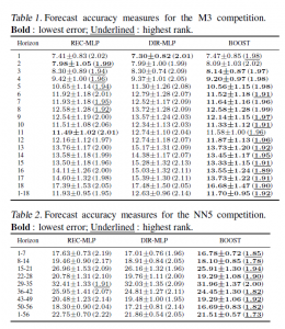
In Boosting multi-step autoregressive forecasts, (Souhaib Ben Taieb and Rob J Hyndman, International Conference on Machine Learning (ICML) 2014) we find the following Table applying boosted time series forecasts to two forecasting competition datasets –

HyndmanTable1

The three columns refer to three methods for generating forecasts over horizons of 1-18 periods (M3 Competition and 1-56 period (Neural Network Competition). The column labeled BOOST is, as its name suggests, the error metric for a boosted time series prediction. Either by the lowest symmetric mean absolute percentage error or a rank criterion, BOOST usually outperforms forecasts produced recursively from an autoregressive (AR) model, or forecasts from an AR model directly mapped onto the different forecast horizons.

There were a lot of empirical time series involved in these two datasets –

The M3 competition dataset consists of 3003 monthly, quarterly, and annual time series. The time series of the M3 competition have a variety of features. Some have a seasonal component, some possess a trend, and some are just fluctuating around some level. The length of the time series ranges between 14 and 126. We have considered time series with a range of lengths between T = 117 and T = 126. So, the number of considered time series turns out to be M = 339. For these time series, the competition required forecasts for the next H = 18 months, using the given historical data. The NN5 competition dataset comprises M = 111 time series representing roughly two years of daily cash withdrawals (T = 735 observations) at ATM machines at one of the various cities in the UK. For each time series, the  competition required to forecast the values of the next H = 56 days (8 weeks), using the given historical data.

This research, notice of which can be downloaded from Rob Hyndman’s site, builds on the methodology of Ben Taieb and Hyndman’s recent paper in the International Journal of Forecasting A gradient boosting approach to the Kaggle load forecasting competition. Ben Taieb and Hyndman’s submission came in 5th out of 105 participating teams in this Kaggle electric load forecasting competition, and used boosting algorithms.

Let me mention a third application of boosting to time series, this one from Germany. So we have Robinzonov, Tutz, and Hothorn’s Boosting Techniques for Nonlinear Time Series Models (Technical Report Number 075, 2010 Department of Statistics University of Munich) which focuses on several synthetic time series and predictions of German industrial production.

Again, boosted time series models comes out well in comparisons.

GErmanIndustrialProd

GLMBoost or GAMBoost are quite competitive at these three forecast horizons for German industrial production.

What is Boosting?

My presentation here is a little “black box” in exposition, because boosting is, indeed, mathematically intricate, although it can be explained fairly easily at a very general level.

Weak predictors and weak learners play an important role in bagging and boosting –techniques which are only now making their way into forecasting and business analytics, although the machine learning community has been discussing them for more than two decades.

Machine learning must be a fascinating field. For example, analysts can formulate really general problems –

In an early paper, Kearns and Valiant proposed the notion of a weak learning algorithm which need only achieve some error rate bounded away from 1/2 and posed the question of whether weak and strong learning are equivalent for efficient (polynomial time) learning algorithms.

So we get the “definition” of boosting in general terms:

Boosting algorithms are procedures that “boost” low-accuracy weak learning algorithms to achieve arbitrarily high accuracy.

And a weak learner is a learning method that achieves only slightly better than chance correct classification of binary outcomes or labeling.

This sounds like the best thing since sliced bread.

But there’s more.

For example, boosting can be understood as a functional gradient descent algorithm.

Now I need to mention that some of the most spectacular achievements in boosting come in classification. A key text is the recent book Boosting: Foundations and Algorithms (Adaptive Computation and Machine Learning series) by Robert E. Schapire and Yoav Freund. This is a very readable book focusing on AdaBoost, one of the early methods and its extensions. The book can be read on Kindle and is starts out –

boostingquote

So worth the twenty bucks or so for the download.

The papers discussed above vis a vis boosting time series apply p-splines in an effort to estimate nonlinear effects in time series. This is really unfamiliar to most of us in the conventional econometrics and forecasting communities, so we have to start conceptualizing stuff like “knots” and component-wise fitting algortihms.

Fortunately, there is a canned package for doing a lot of the grunt work in R, called mboost.

Bottom line, I really don’t think time series analysis will ever be the same.