Category Archives: data science

Links – Data Science

I’ve always thought the idea of “data science” was pretty exciting. But what is it, how should organizations proceed when they want to hire “data scientists,” and what’s the potential here?

Clearly, data science is intimately associated with Big Data. Modern semiconductor and computer technology make possible rich harvests of “bits” and “bytes,” stored in vast server farms. Almost every personal interaction can be monitored, recorded, and stored for some possibly fiendish future use, along with what you might call “demographics.” Who are you? Where do you live? Who are your neighbors and friends? Where do you work? How much money do you make? What are your interests, and what websites do you browse? And so forth.

As Edward Snowden and others point out, there is a dark side. It’s possible, for example, all phone conversations are captured as data flows and stored somewhere in Utah for future analysis by intrepid…yes, that’s right…data scientists.

In any case, the opportunities for using all this data to influence buying decisions, decide how to proceed in business, to develop systems to “nudge” people to do the right thing (stop smoking, lose weight), and, as I have recently discovered – do good, are vast and growing. And I have not even mentioned the exploding genetics data from DNA arrays and its mobilization to, for example, target cancer treatment.

The growing body of methods and procedures to make sense of this extensive and disparate data is properly called “data science.” It’s the blind man and the elephant problem. You have thousands or millions of rows of cases, perhaps with thousands or even millions of columns representing measurable variables. How do you organize a search to find key patterns which are going to tell your sponsors how to do what they do better?

Hiring a Data Scientist

Companies wanting to “get ahead of the curve” are hiring data scientists – from positions as illustrious and mysterious as Chief Data Scientist to operators in what are almost now data sweatshops.

But how do you hire a data scientist if universities are not granting that degree yet, and may even be short courses on “data science?”

I found a terrific article – How to Consistently Hire Remarkable Data Scientists.

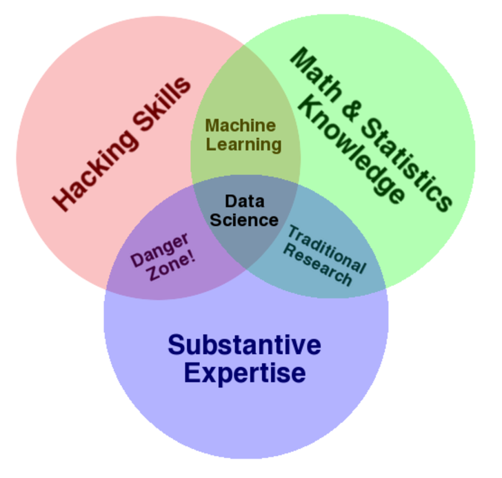
It cites Drew Conway’s data science Venn Diagram suggesting where data science falls in these intersecting areas of knowledge and expertise.

DataScienceVenn

This article, which I first found in a snappy new compilation Data Elixir also highlights methods used by Alan Turing to recruit talent at Benchley.

In the movie The Imitation Game, Alan Turing’s management skills nearly derail the British counter-intelligence effort to crack the German Enigma encryption machine. By the time he realized he needed help, he’d already alienated the team at Bletchley Park. However, in a moment of brilliance characteristic of the famed computer scientist, Turing developed a radically different way to recruit new team members.

To build out his team, Turing begins his search for new talent by publishing a crossword puzzle in The London Daily Telegraph inviting anyone who could complete the puzzle in less than 12 minutes to apply for a mystery position. Successful candidates were assembled in a room and given a timed test that challenged their mathematical and problem solving skills in a controlled environment. At the end of this test, Turing made offers to two out of around 30 candidates who performed best.

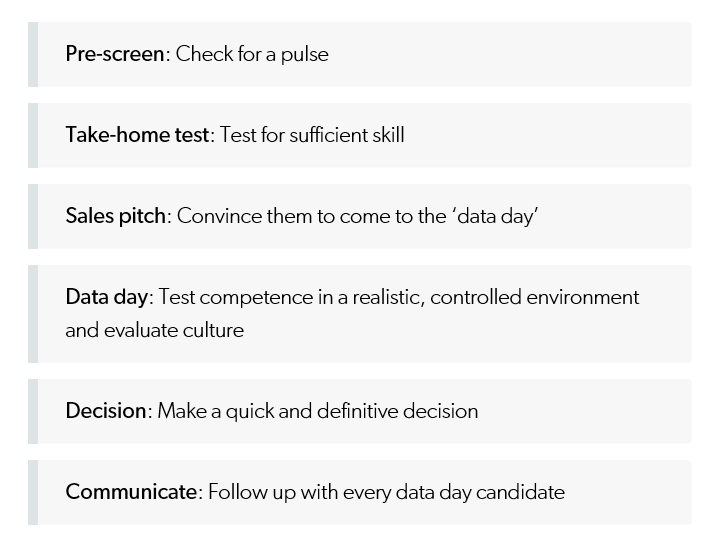
In any case, the recommendation is a six step process to replace the traditional job interview –

SixStageHiringTest

Doing Good With Data Science

Drew Conway, the author of the Venn Diagram shown above, is associated with a new kind of data company called Data Kind.

Here’s an entertaining video of Conway, an excellent presenter, discussing Big Data as a movement and as something which can be used for social good.

For additional detail see http://venturebeat.com/2014/08/21/datakinds-benevolent-data-science-projects-arrive-in-5-more-cities/
Behavioral Economics and Holiday Gifts

Chapter 1 of Advances in Behavioral Economics highlights the core proposition of this emerging field – namely that real economic choices over risky outcomes do not conform to the expected utility (EU) hypothesis.

The EU hypothesis states that the utility of a risky distribution of outcomes is a probability-weighted average of the outcome utilities. Many violations of this principle are demonstrated with psychological experiments.

These violations suggest “nudge” theory – that small, apparently inconsequential changes in the things people use can have disproportionate effects on behavior.

Along these lines, I found this PBS report by Paul Solman fascinating. In it, Solman, PBS economics correspondent, talks to Sendhil Mullainathan at Harvard University about consumer innovations that promise to improve your life through behavioral economics – and can be gifts for this Season. 

Happy Holidays all. 

Stylized Facts About Stock Market Volatility

Volatility of stock market returns is more predictable, in several senses, than stock market returns themselves.

Generally, if pt is the price of a stock at time t, stock market returns often are defined as ln(pt)-ln(pt-1). Volatility can be the absolute value of these returns, or as their square. Thus, hourly, daily, monthly or other returns can be positive or negative, while volatility is always positive.

Masset highlights several stylized facts about volatility in a recent paper –

  • Volatility is not constant and tends to cluster through time. Observing a large (small) return today (whatever its sign) is a good precursor of large (small) returns in the coming days.
  • Changes in volatility typically have a very long-lasting impact on its subsequent evolution. We say that volatility has a long memory.
  • The probability of observing an extreme event (either a dramatic downturn or an enthusiastic takeoff) is way larger than what is hypothesized by common data generating processes. The returns distribution has fat tails.
  • Such a shock also has a significant impact on subsequent returns. Like in an earthquake, we typically observe aftershocks during a number of trading days after the main shock has taken place.
  • The amplitude of returns displays an intriguing relation with the returns themselves: when prices go down – volatility increases; when prices go up – volatility decreases but to a lesser extent. This is known as the leverage effect … or the asymmetric volatility phenomenon.
  • Recently, some researchers have noticed that there were also some significant differences in terms of information content among volatility estimates computed at various frequencies. Changes in low-frequency volatility have more impact on subsequent high-frequency volatility than the opposite. This is due to the heterogeneous nature of market participants, some having short-, medium- or long-term investment horizons, but all being influenced by long-term moves on the markets…
  • Furthermore, … the intensity of this relation between long and short time horizons depends on the level of volatility at long horizons: when volatility at a long time horizon is low, this typically leads to low volatility at short horizons too. The reverse is however not always true…

Masset extends and deepens this type of result for bull and bear markets and developed/emerging markets. Generally, emerging markets display higher volatility with some differences in third and higher moments.

A key reference is Rami Cont’s Empirical properties of asset returns: stylized facts and statistical issues which provides this list of features of stock market returns, some of which directly relate to volatility. This is one of the most widely-cited articles in the financial literature:

  1. Absence of autocorrelations: (linear) autocorrelations of asset returns are often insignificant, except for very small intraday time scales (~20 minutes) for which microstructure effects come into play.
  2. Heavy tails: the (unconditional) distribution of returns seems to display a power-law or Pareto-like tail, with a tail index which is finite, higher than two and less than five for most data sets studied. In particular this excludes stable laws with infinite variance and the normal distribution. However the precise form of the tails is difficult to determine.
  3. Gain/loss asymmetry: one observes large drawdowns in stock prices and stock index values but not equally large upward movements.
  4. Aggregational Gaussianity: as one increases the time scale t over which returns are calculated, their distribution looks more and more like a normal distribution. In particular, the shape of the distribution is not the same at different time scales.
  5. Intermittency: returns display, at any time scale, a high degree of variability. This is quantified by the presence of irregular bursts in time series of a wide variety of volatility estimators.
  6. Volatility clustering: different measures of volatility display a positive autocorrelation over several days, which quantifies the fact that high-volatility events tend to cluster in time.
  7. Conditional heavy tails: even after correcting returns for volatility clustering (e.g. via GARCH-type models), the residual time series still exhibit heavy tails. However, the tails are less heavy than in the unconditional distribution of returns.
  8. Slow decay of autocorrelation in absolute returns: the autocorrelation function of absolute returns decays slowly as a function of the time lag, roughly as a power law with an exponent β ∈ [0.2, 0.4]. This is sometimes interpreted as a sign of long-range dependence.
  9. Leverage effect: most measures of volatility of an asset are negatively correlated with the returns of that asset.
  10. Volume/volatility correlation: trading volume is correlated with all measures of volatility.
  11. Asymmetry in time scales: coarse-grained measures of volatility predict fine-scale volatility better than the other way round.

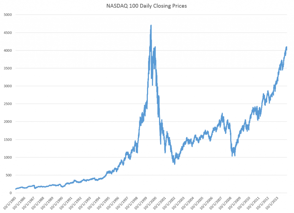
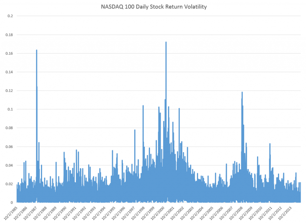
Just to position the discussion, here are graphs of the NASDAQ 100 daily closing prices and the volatility of daily returns, since October 1, 1985.

NASDAQ100new

The volatility here is calculated as the absolute value of the differences of the logarithms of the daily closing prices.

NASDAQ100V

Links – mid-September

After highlighting billionaires by state, I focus on data analytics and marketing, and then IT in these links. Enjoy!

The Wealthiest Individual In Every State [Map]

wealthyindividuals

Data Analytics and Marketing

A Predictive Analytics Primer

Has your company, for example, developed a customer lifetime value (CLTV) measure? That’s using predictive analytics to determine how much a customer will buy from the company over time. Do you have a “next best offer” or product recommendation capability? That’s an analytical prediction of the product or service that your customer is most likely to buy next. Have you made a forecast of next quarter’s sales? Used digital marketing models to determine what ad to place on what publisher’s site? All of these are forms of predictive analytics.

Making sense of Google Analytics audience data

Earlier this year, Google added Demographics and Interest reports to the Audience section of Google Analytics (GA). Now not only can you see how many people are visiting your site, but how old they are, whether they’re male or female, what their interests are, and what they’re in the market for.

Data Visualization, Big Data, and the Quest for Better Decisions – a Synopsis

Simon uses Netflix as a prime example of a company that gets data and its use “to promote experimentation, discovery, and data-informed decision-making among its people.”….

They know a lot about their customers.

For example, the company knows how many people binge-watched the entire season four of Breaking Bad the day before season five came out (50,000 people). The company therefore can extrapolate viewing patterns for its original content produced to appeal to Breaking Bad fans. Moreover, Netflix markets the same show differently to different customers based on whether their viewing history suggests they like the director or one of the stars….

The crux of their analytics is the visualization of “what each streaming customer watches, when, and on what devices, but also at what points shows are paused and resumed (or not) and even the color schemes of the marketing graphics to which individuals respond.”

How to Market Test a New Idea

Formulate a hypothesis to be tested. Determine specific objectives for the test. Make a prediction, even if it is just a wild guess, as to what should happen. Then execute in a way that enables you to accurately measure your prediction…Then involve a dispassionate outsider in the process, ideally one who has learned through experience how to handle decisions with imperfect information…..Avoid considering an idea in isolation. In the absence of choice, you will almost always be able to develop a compelling argument about why to proceed with an innovation project. So instead of asking whether you should invest in a specific project, ask if you are more excited about investing in Project X versus other alternatives in your innovation portfolio…And finally, ensure there is some kind of constraint forcing a decision.

Information Technology (IT)

5 Reasons why Wireless Charging Never Caught on

Charger Bundling, Limited handsets, Time, Portability, and Standardisation – interesting case study topic for IT

Why Jimmy the Robot Means New Opportunities for IT

While Jimmy was created initially for kids, the platform is actually already evolving to be a training platform for everyone. There are two versions: one at $1,600, which really is more focused on kids, and one at $16,000, for folks like us who need a more industrial-grade solution. The Apple I wasn’t just for kids and neither is Jimmy. Consider at least monitoring this effort, if not embracing it, so when robots go vertical you have the skills to ride this wave and not be hit by it.

jimmy-the-robot

Beyond the Reality Distortion Field: A Sober Look at Apple Pay

.. Apple Pay could potentially kick-start the mobile payment business the way the iPod and iTunes launched mobile music 13 years ago. Once again, Apple is leveraging its powerful brand image to bring disparate companies together all in the name of consumer convenience.

From Dr. 4Ward How To Influence And Persuade (click to enlarge)

influence

Ebola and Data Analysis

Data analysis and predictive analytics can support national and international responses to ebola.

One of the primary ways at present is by verifying and extrapolating the currently exponential growth of ebola in affected areas – especially in Monrovia, the capital of Liberia, as well as Sierra Leone, Guinea, Nigeria, and the Democratic Republic of the Congo.

At this point, given data from the World Health Organization (WHO) and other agencies, predictive modeling can be as simple as in the following two charts, developed from the data compiled (and documented) in the Wikipedia site.

The first charts datapoints from the end of the months of May through August of this year.

Ebolacasesmodeling

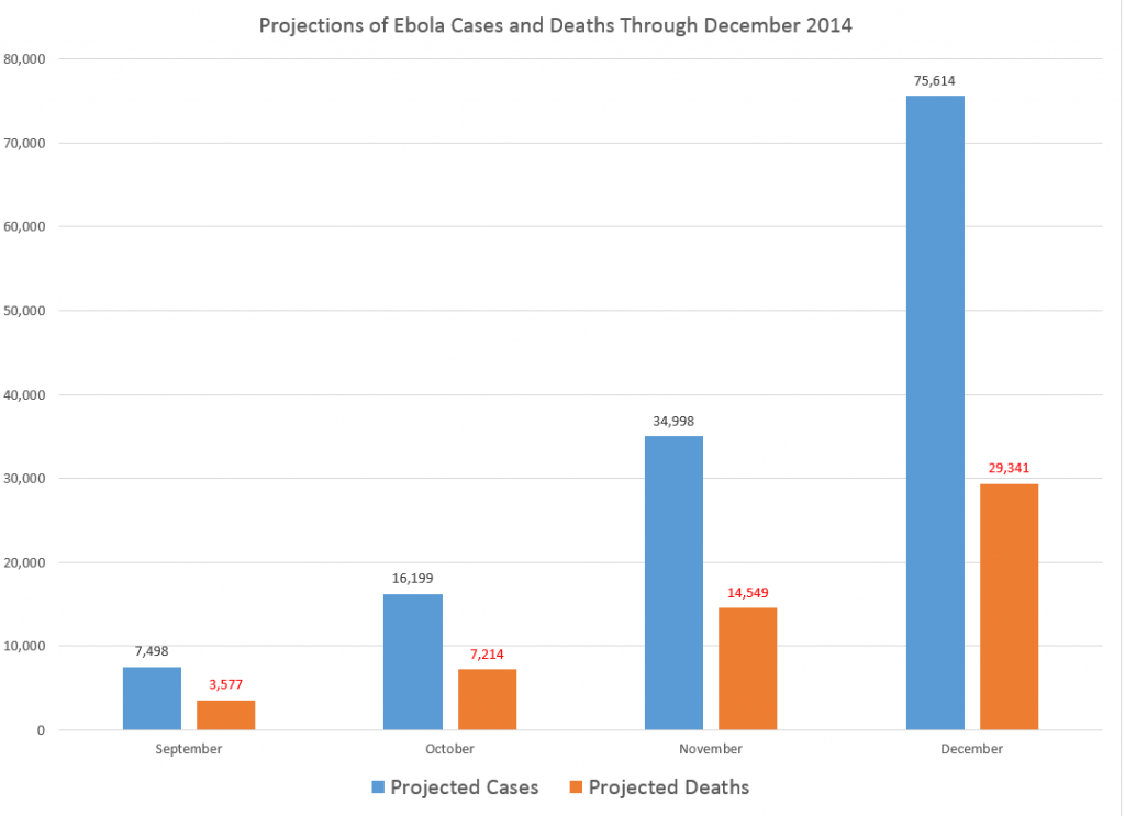
The second chart extrapolates an exponential fit to these cases, shown in the lines in the above figure, by month through December 2014.

Ebolaprojections

So by the end of this year, if this epidemic courses unchecked, without the major public health investments necessary in terms of hospital beds, supplies, medical and supporting personnel, including military or police forces to maintain public order in some of the worst-hit areas – there will be nearly 80,000 cases and approximately 30,000 deaths, by this simple extrapolation.

A slightly more sophisticated analysis by Geert Barentsen, utilizing data within calendar months as well, concludes that currently Ebola cases have a doubling time of 29 days.

One possibly positive aspect of these projections is the death rate declines from around 60 to 40 percent, from May through December 2014.

However, if the epidemic continues through 2015 at this rate, the projections suggest there will be more than 300 million cases.

World Health Organization (WHO) estimates released the first week of September indicate nearly 2,400 deaths. Total numbers of cases from the same period in early September is 4,846. So the projections are on track so far.

And, if you wish, you can validate these crude data analytics with reference to modeling using the classic compartment approach and other more advanced setups. See, for example, Disease modelers project a rapidly rising toll from Ebola or the recent New York Times article.

Visual Analytics

There have been advanced modeling efforts at discovering the possibilities of transmission of Ebola through persons traveling by air to other affected areas.

Here is a chart from Assessing the International Spreading Risk Associated with the 2014 West African Ebola Outbreak.

ebolaairroutes

As a data and forecasting analyst, I am not specially equipped to comment on the conditions which make transmission of this disease particularly dangerous. But I think, to some extent, it’s not rocket science.

Crowded conditions in many African cities, low educational attainment, poverty, poor medical infrastructure, rapid population growth – all these factors contribute to the high basic reproductive number of the disease in this outbreak. And, if the numbers of cases increase toward 100,000, the probability that some of the affected individuals will travel elsewhere grows, particularly when efforts to quarantine areas seem heavy-handed and, given little understanding of modern disease models in the affected populations, possibly suspicious.

There is a growing response from agencies and places as widely ranging as the Gates Foundation and Cuba, but what I read is that a military-type operation will be necessary to bring the epidemic under control. I suppose this means command-and-control centers must be established, set procedures must be implemented when cases are identified, adequate field hospitals need to be established, enough medical personnel must be deployed, and so forth. And if there are potential vaccines, these probably will be expensive to administer in early stages.

These thoughts are suggested by the numbers. So far, the numbers speak for themselves.

Links – Labor Day Weekend

Tech

Amazon’s Cloud Is So Pervasive, Even Apple Uses It

Your iCloud storage is apparently on Amazon.

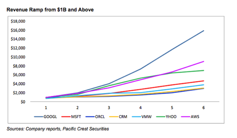
Amazon’s Cloud Is The Fastest Growing Software Business In History

AWS

AWS is Amazon Web Services. The author discounts Google growth, since it is primarily a result of selling advertising. 

How Microsoft and Apple’s Ads Define Their Strategy

Microsoft approaches the market from the top down, while Apple goes after the market from the bottom up.

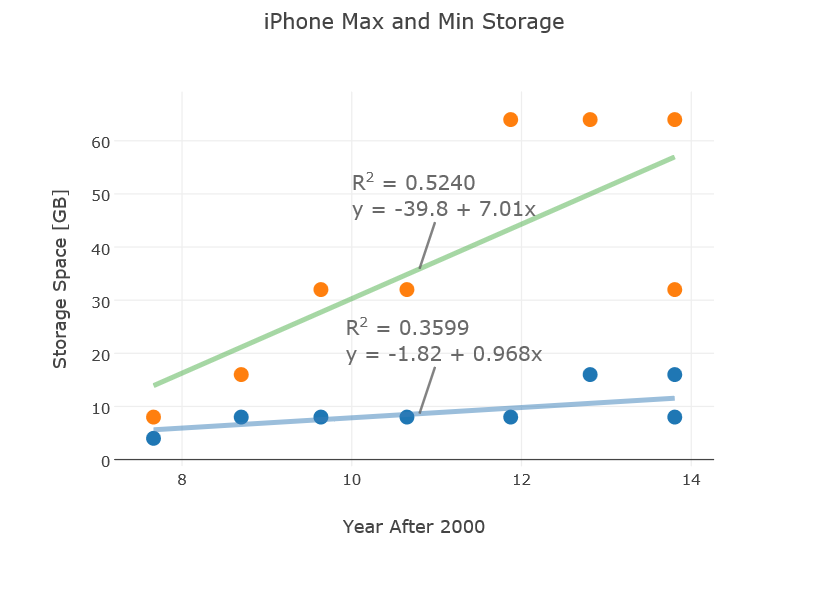
Mathematical Predictions for the iPhone 6

Can you predict features of the iPhone6 scheduled to be released September 6?

iphoneplot

Predictive Analytics

Comparison of statistical software

Good links for R, Matlab, SAS, Stata, and SPSS.

Types and Uses of Predictive Analytics, What they are and Where You Can Put Them to Work

Gartner says that predictive analytics is a mature technology yet only one company in eight is currently utilizing this ability to predict the future of sales, finance, production, and virtually every other area of the enterprise. What is the promise of predictive analytics and what exactly are they [types and uses of predictive analytics]? Good highlighting of main uses of predictive analytics in companies.

The Four Traps of Predictive Analytics

Magical thinking/ Starting at the Top/ Building Cottages, not Factories/ Seeking Purified Data. Good discussion. This short article in the Sloan Management Review is spot on, in my opinion. The way to develop good predictive analytics is to pick an area, indeed, pick the “low-handing fruit.” Develop workable applications, use them, improve them, broaden the scope. The “throw everything including the kitchen sink” approach of some early Big Data deployments is almost bound to fail. Flashy, trendy, but, in the final analysis, using “exhaust data” to come up with obscure customer metrics probably will not cut in the longer run.

Economic Issues

The Secular Stagnation Controversy

– discusses the e-book Secular Stagnation: Facts, Causes and Cures. The blogger Timothy Taylor points out that “secular” here has no relationship to lacking a religious context, but refers to the idea that market economies, or, if you like, capitalist economies, can experience long periods (decade or more) of desultory economic growth. Check the e-book for Larry Summer’s latest take on the secular stagnation hypothesis.

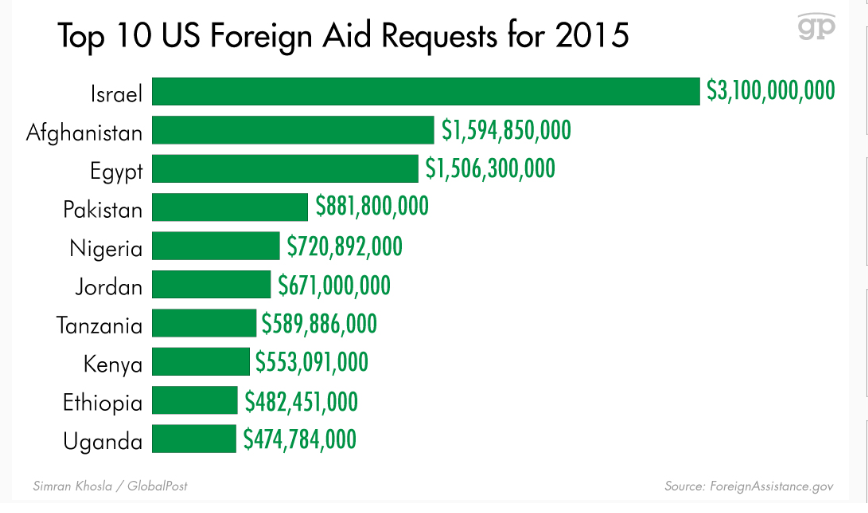
Here’s how much aid the US wants to send foreign countries in 2015, and why (INFOGRAPHIC

foreignaid

First peek at “Revolutions” exhibit at Computer History Museum with Woz

I think Steve Wozniack is a kind of hero – from what I understand still connected with helping young people and in this video, giving some “straight from the horses mouth” commentary on the history of computing. 

And I am making plans to return to pattern on this blog.

That is, I will be focusing on issues tagged a couple of posts ago – namely geopolitical risks (ebola, unfolding warfare at several locations), the emerging financial bubble, and 21st century data analysis and forecasting techniques.

But, I think perhaps a little like Woz, I am a technological utopian at heart. If we could develop technologies which would allow younger people around the globe some type of “hands on” potential – maybe a little like the old computer systems which these technical leaders, now mostly all billionaires, had access to – if we could find these new technologies, I think we could knit the world together once again. Of course, this idea devolves when the “hands on” potential is occasioned by weapons – and the image of the child soldiers in Africa comes to mind.

I like the part in the video where Woz describes using a nonstandard card punch machine to get his card deck in order at Berkeley – the part where he draws a lesson about learning to do what works, not what the symbols indicate.

Some Cycle Basics

A Fourier analysis is one of the first steps in analyzing cycles.

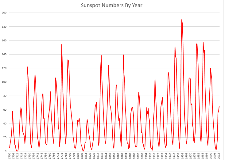
Take sunspots, for example,

There are extensive historic records on the annual number of sunspots, dating back to 1700. The annual data shown in the following graph dates back to 1700, and is currently maintained by the Royal Belgium Observatory.

sunspots

This series is relatively stationary, although there may be a slight trend if you cut this span of data off a few years before the present.

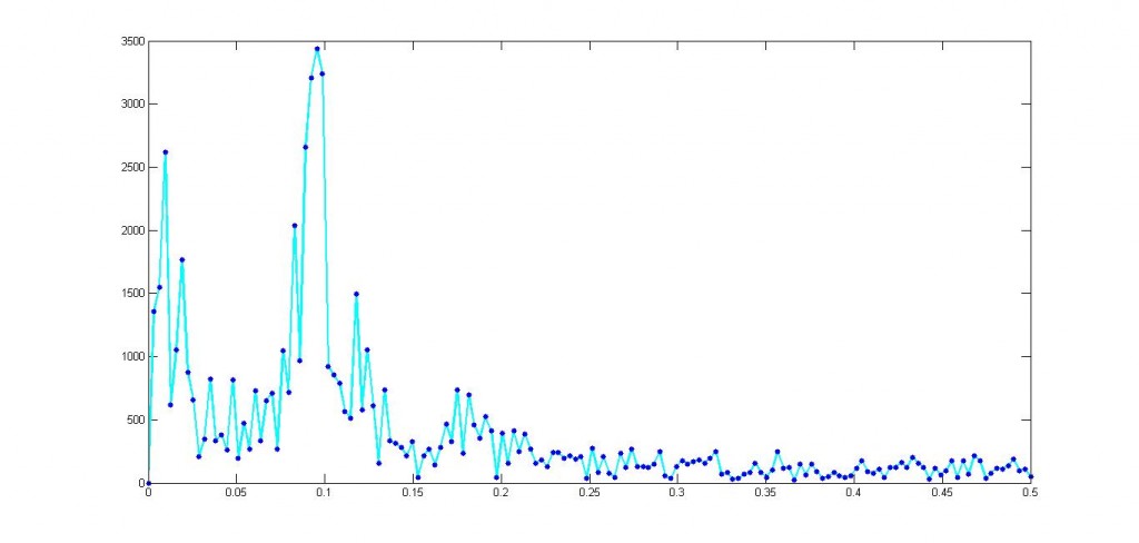
In any case, the kind of thing you get with a Fourier analysis looks like this.

spectralsunspots

This shows the power or importance of the cycles/year numbers, and maxes out at around 0.09.

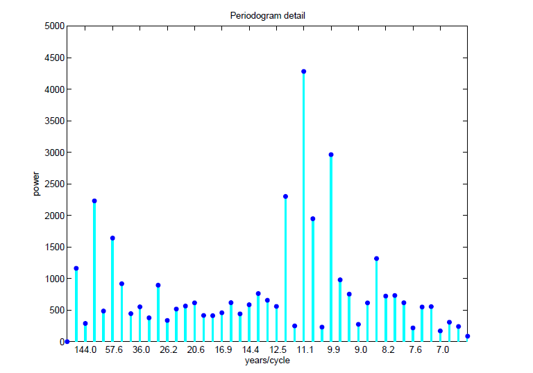
These data can be recalibrated into the following chart, which highlights the approximately 11 year major cycle in the sunspot numbers.

sunspotsperiodogramyr

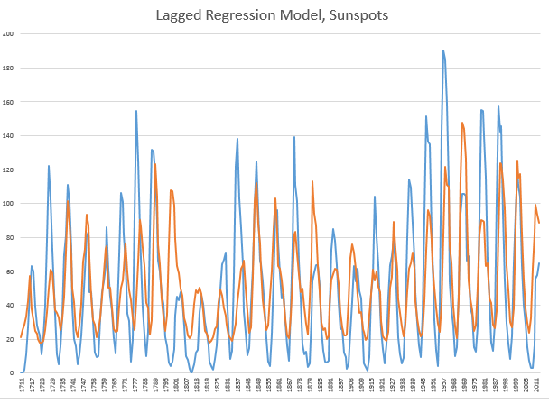
Now it’s possible to build a simple regression model with a lagged explanatory variable to make credible predictions. A lag of eleven years produces the following in-sample and out-of-sample fits. The regression is estimated over data to 1990, and, thus, the years 1991 through 2013 are out-of-sample.

LaggedModel

It’s obvious this sort of forecasting approach is not quite ready for prime-time television, even though it performs OK on several of the out-of-sample years after 1990.

But this exercise does highlight a couple of things.

First, the annual number of sunspots is broadly cyclical in this sense. If you try the same trick with lagged values for the US “business cycle” the results will be radically worse. At least with the sunspot data, most of the fluctuations have timing that is correctly predicted, both in-sample (1990 and before) and out-of-sample (1991-2013).

Secondly, there are stochastic elements to this solar activity cycle. The variation in amplitude is dramatic, and, indeed, the latest numbers coming in on sunspot activity are moving to much lower levels, even though the cycle is supposedly at its peak.

I’ve reviewed several papers on predicting the sunspot cycle. There are models which are more profoundly inspired by the possible physics involved – dynamo dynamics for example. But for my money there are basic models which, on a one-year-ahead basis, do a credible job. More on this forthcoming.

Video Friday – Andrew Ng’s Machine Learning Course

Well, I signed up for Andrew Ng’s Machine Learning Course at Stanford. It began a few weeks ago, and is a next generation to lectures by Ng circulating on YouTube. I’m going to basically audit the course, since I started a little late, but I plan to take several of the exams and work up a few of the projects. This course provides a broad introduction to machine learning, datamining, and statistical pattern recognition. Topics include: (i) Supervised learning (parametric/non-parametric algorithms, support vector machines, kernels, neural networks). (ii) Unsupervised learning (clustering, dimensionality reduction, recommender systems, deep learning). (iii) Best practices in machine learning (bias/variance theory; innovation process in machine learning and AI). The course will also draw from numerous case studies and applications, so that you’ll also learn how to apply learning algorithms to building smart robots (perception, control), text understanding (web search, anti-spam), computer vision, medical informatics, audio, database mining, and other areas. I like the change in format. The YouTube videos circulating on the web are lengthly, and involve Ng doing derivations on white boards. This is a more informal, expository format. Here is a link to a great short introduction to neural networks. Ngrobot Click on the link above this picture, since the picture itself does not trigger a YouTube. Ng’s introduction on this topic is fairly short, so here is the follow-on lecture, which starts the task of representing or modeling neural networks. I really like the way Ng approaches this is grounded in biology. I believe there is still time to sign up. Comment on Neural Networks and Machine Learning I can’t do much better than point to Professor Ng’s definition of machine learning – Machine learning is the science of getting computers to act without being explicitly programmed. In the past decade, machine learning has given us self-driving cars, practical speech recognition, effective web search, and a vastly improved understanding of the human genome. Machine learning is so pervasive today that you probably use it dozens of times a day without knowing it. Many researchers also think it is the best way to make progress towards human-level AI. In this class, you will learn about the most effective machine learning techniques, and gain practice implementing them and getting them to work for yourself. More importantly, you’ll learn about not only the theoretical underpinnings of learning, but also gain the practical know-how needed to quickly and powerfully apply these techniques to new problems. Finally, you’ll learn about some of Silicon Valley’s best practices in innovation as it pertains to machine learning and AI. And now maybe this is the future – the robot rock band.

Wrap on Exponential Smoothing

Here are some notes on essential features of exponential smoothing.

  1. Name. Exponential smoothing (ES) algorithms create exponentially weighted sums of past values to produce the next (and subsequent period) forecasts. So, in simple exponential smoothing, the recursion formula is Lt=αXt+(1-α)Lt-1 where α is the smoothing constant constrained to be within the interval [0,1], Xt is the value of the time series to be forecast in period t, and Lt is the (unobserved) level of the series at period t. Substituting the similar expression for Lt-1 we get Lt=αXt+(1-α) (αXt-1+(1-α)Lt-2)= αXt+α(1-α)Xt-1+(1-α)2Lt-2, and so forth back to L1. This means that more recent values of the time series X are weighted more heavily than values at more distant times in the past. Incidentally, the initial level L1 is not strongly determined, but is established by one ad hoc means or another – often by keying off of the initial values of the X series in some manner or another. In state space formulations, the initial values of the level, trend, and seasonal effects can be included in the list of parameters to be established by maximum likelihood estimation.
  2. Types of Exponential Smoothing Models. ES pivots on a decomposition of time series into level, trend, and seasonal effects. Altogether, there are fifteen ES methods. Each model incorporates a level with the differences coming as to whether the trend and seasonal components or effects exist and whether they are additive or multiplicative; also whether they are damped. In addition to simple exponential smoothing, Holt or two parameter exponential smoothing is another commonly applied model. There are two recursion equations, one for the level Lt and another for the trend Tt, as in the additive formulation, Lt=αXt+(1-α)(Lt-1+Tt-1) and Tt=β(Lt– Lt-1)+(1-β)Tt-1 Here, there are now two smoothing parameters, α and β, each constrained to be in the closed interval [0,1]. Winters or three parameter exponential smoothing, which incorporates seasonal effects, is another popular ES model.
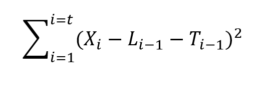
  3. Estimation of the Smoothing Parameters. The original method of estimating the smoothing parameters was to guess their values, following guidelines like “if the smoothing parameter is near 1, past values will be discounted further” and so forth. Thus, if the time series to be forecast was very erratic or variable, a value of the smoothing parameter which was closer to zero might be selected, to achieve a longer period average. The next step is to set up a sum of the squared differences of the within sample predictions and minimize these. Note that the predicted value of Xt+1 in the Holt or two parameter additive case is Lt+Tt, so this involves minimizing the expression Sqerroreq Currently, the most advanced method of estimating the value of the smoothing parameters is to express the model equations in state space form and utilize maximum likelihood estimation. It’s interesting, in this regard, that the error correction version of ES recursion equations are a bridge to this approach, since the error correction formulation is found at the very beginnings of the technique. Advantages of using the state space formulation and maximum likelihood estimation include (a) the ability to estimate confidence intervals for point forecasts, and (b) the capability of extending ES methods to nonlinear models.
  4. Comparison with Box-Jenkins or ARIMA models. ES began as a purely applied method developed for the US Navy, and for a long time was considered an ad hoc procedure. It produced forecasts, but no confidence intervals. In fact, statistical considerations did not enter into the estimation of the smoothing parameters at all, it seemed. That perspective has now changed, and the question is not whether ES has statistical foundations – state space models seem to have solved that. Instead, the tricky issue is to delineate the overlap and differences between ES and ARIMA models. For example, Gardner makes the statement that all linear exponential smoothing methods have equivalent ARIMA models. Hyndman points out that the state space formulation of ES models opens the way for expressing nonlinear time series – a step that goes beyond what is possible in ARIMA modeling.
  5. The Importance of Random Walks. The random walk is a forecasting benchmark. In an early paper, Muth showed that a simple exponential smoothing model provided optimal forecasts for a random walk. The optimal forecast for a simple random walk is the current period value. Things get more complicated when there is an error associated with the latent variable (the level). In that case, the smoothing parameter determines how much of the recent past is allowed to affect the forecast for the next period value.
  6. Random Walks With Drift. A random walk with drift, for which a two parameter ES model can be optimal, is an important form insofar as many business and economic time series appear to be random walks with drift. Thus, first differencing removes the trend, leaving ideally white noise. A huge amount of ink has been spilled in econometric investigations of “unit roots” – essentially exploring whether random walks and random walks with drift are pretty much the whole story when it comes to major economic and business time series.
  7. Advantages of ES. ES is relatively robust, compared with ARIMA models, which are sensitive to mis-specification. Another advantage of ES is that ES forecasts can be up and running with only a few historic observations. This comment applied to estimation of the level and possibly trend, but does not apply in the same degree to the seasonal effects, which usually require more data to establish. There are a number of references which establish the competitive advantage in terms of the accuracy of ES forecasts in a variety of contexts.
  8. Advanced Applications.The most advanced application of ES I have seen is the research paper by Hyndman et al relating to bagging exponential smoothing forecasts.

The bottom line is that anybody interested in and representing competency in business forecasting should spend some time studying the various types of exponential smoothing and the various means to arrive at estimates of their parameters.

For some reason, exponential smoothing reaches deep into actual process in data generation and consistently produces valuable insights into outcomes.