Category Archives: new proximity model

Out-Of-Sample R2 Values for PVAR Models

Out-of-sample (OOS) R2 is a good metric to apply to test whether your predictive relationship has out-of-sample predictability. Checking this for the version of the proximity variable model which is publically documented, I find OOS R2 of 0.63 for forecasts of daily high prices.

In other words, 63 percent of the variation of the daily growth in high prices for the S&P 500 is explained by four variables, documented in Predictability of the Daily High and Low of the S&P 500 Index.

This is a really high figure for any kind of predictive relationship involving security prices, so I thought I would put the data out there for anyone interested to check.

OOS R2

This metric is often found in connection with efforts to predict daily or other rates of return on securities, and is commonly defined as

OOSR2

See, for example, Campbell and Thompson.

The white paper linked above and downloadable from University of Munich archives shows –

Ratios involving the current period opening price and the high or low price of the previous period are significant predictors of the current period high or low price for many stocks and stock indexes. This is illustrated with daily trading data from the S&P 500 index. Regressions specifying these “proximity variables” have higher explanatory and predictive power than benchmark autoregressive and “no change” models. This is shown with out-of-sample comparisons of MAPE, MSE, and the proportion of time models predict the correct direction or sign of change of daily high and low stock prices. In addition, predictive models incorporating these proximity variables show time varying effects over the study period, 2000 to February 2015. This time variation looks to be more than random and probably relates to investor risk preferences and changes in the general climate of investment risk.

I wanted to provide interested readers with a spreadsheet containing the basic data and computations of this model, which I call the “proximity variable” model. The idea is that the key variables are ratios of nearby values.

And this is sort of an experiment, since I have not previously put up a spreadsheet for downloading on this blog. And please note the spreadsheet data linked below is somewhat different than the original data for the white paper, chiefly by having more recent observations. This does change the parameter estimates for the whole sample, since the paper shows we are in the realm of time-varying coefficients.

So here goes. Check out this link. PVARresponse

Of course, no spreadsheet is totally self-explanatory, so a few words.

First, the price data (open, high, low, etc) for the S&P 500 come from Yahoo Finance, although the original paper used other sources, too.

Secondly, the data matrix for the regressions is highlighted in light blue. The first few rows of this data matrix include the formulas with later rows being converted to numbers, to reduce the size of the file.

If you look in column K below about row 1720, you will find out-of-sample regression forecasts, created by using data from the immediately preceding trading day and before and current day opening price ratios.

There are 35 cases, I believe, in which the high of the day and the opening price are the same. These can easily be eliminated in calculating any metrics, and, doing so, in fact increases the OOS R2.

I’m sympathetic with readers who develop a passion to “show this guy to be all wrong.” I’ve been there, and it may help to focus on computational matters.

However, there is just no question but this approach is novel, and beats both No Change forecasts and a first order autoregressive forecasts (see the white paper) by a considerable amount.

I personally think these ratios are closely watched by some in the community of traders, and that other price signals motivating trades are variously linked with these variables.

My current research goes further than outlined in the white paper – a lot further. At this point, I am tempted to suggest we are looking at a new paradigm in predictability of stock prices. I project “waves of predictability” will be discovered in the movement of ensembles of security prices. These might be visualized like the wave at a football game, if you will. But the basic point is that I reckon we can show how early predictions of these prices changes are self-confirming to a degree, so emerging signs of the changes being forecast in fact intensify the phenomena being predicted.

Think big.

Keep the comments coming.

One-Month-Ahead Stock Market Forecasts

I have been spending a lot of time analyzing stock market forecast algorithms I stumbled on several months ago which I call the New Proximity Algorithms (NPA’s).

There is a white paper on the University of Munich archive called Predictability of the Daily High and Low of the S&P 500 Index. This provides a snapshot of the NPA at one stage of development, and is rock solid in terms of replicability. For example, an analyst replicated my results with Python, and I’ll probably will provide his code here at some point.

I now have moved on to longer forecast periods and more complex models, and today want to discuss month-ahead forecasts of high and low prices of the S&P 500 for this month – June.

Current Month Forecast for S&P 500

For the current month – June 2015 – things look steady with no topping out or crash in sight

With opening price data from June 1, the NPA month-ahead forecast indicates a high of 2144 and a low of 2030. These are slightly above the high and low for May 2015, 2,134.72 and 2,067.93, respectively.

But, of course, a week of data for June already is in, so, strictly speaking, we need a three week forecast, rather than a forecast for a full month ahead, to be sure of things. And, so far, during June, daily high and low prices have approached the predicted values, already.

In the interests of gaining better understanding of the model, however, I am going to “talk this out” without further computations at this moment.

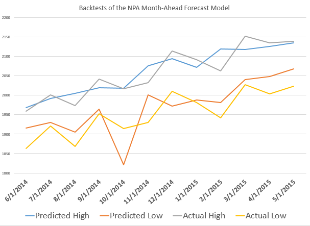
So, one point is that the model for the low is less reliable than the high price forecast on a month-ahead basis. Here, for example, is the track record of the NPA month-ahead forecasts for the past 12 months or so with S&P 500 data.

12MOSNPA

The forecast model for the high tracks along with the actuals within around 1 percent forecast error, plus or minus. The forecast model for the low, however, has a big miss with around 7 percent forecast error in late 2014.

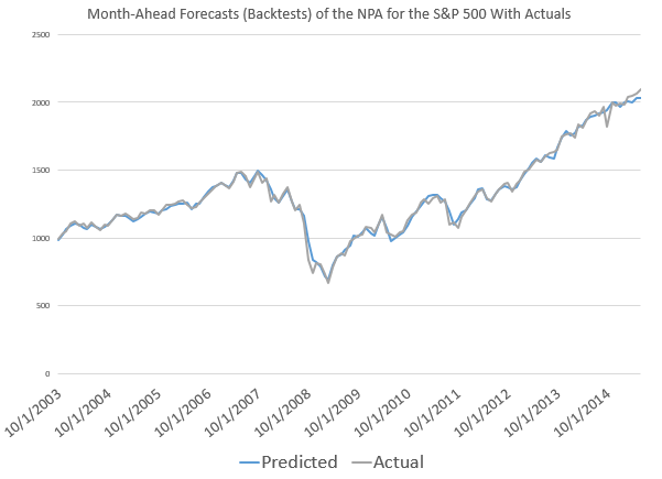
This sort of “wobble” for the NPA forecast of low prices is not unusual, as the following chart, showing backtests to 2003, shows.

LowMonthAheadBig

What’s encouraging is the NPA model for the low price adjusts quickly. If large errors signal a new direction in price movement, the model catches that quickly. More often, the wobble in the actual low prices seems to be transitory.

Predicting Turning Points

One reason why the NPA monthly forecast for June might be significant, is that the underlying method does a good job of predicting major turning points.

If a crash were coming in June, it seems likely, based on backtesting, that the model would signal something more than a slight upward trend in both the high and low prices.

Here are some examples.

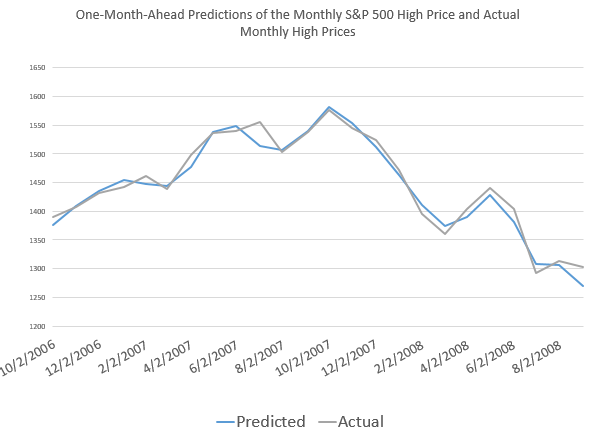
First, the NPA forecast model for the high price of the S&P 500 caught the turning point in 2007 when the market began to go into reverse.

S&P2008high

But that is not all.

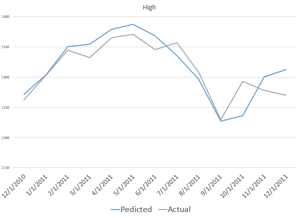
The NPA model for the month-ahead high price also captures a more recent reversal in the S&P 500.

laterHighS&P500


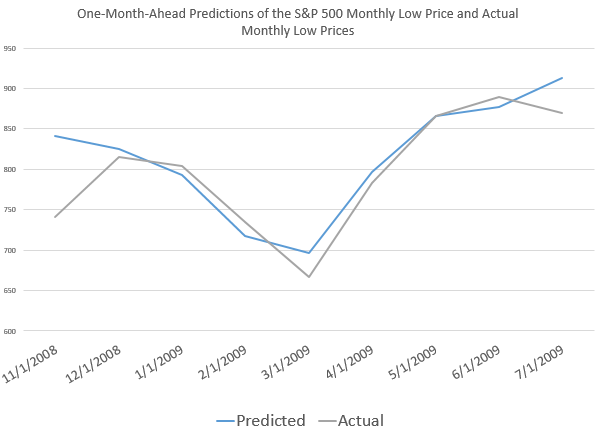
Also, the model for the low did capture the bottom in the S&P 500 in 2009, when the direction of the market changed from decline to increase.

2008High

This type of accuracy in timing in forecast modeling is quite remarkable.

It’s something I also saw earlier with the Hong Kong Hang Seng Index, but which seemed at that stage of model development to be confined to Chinese market data.

Now I am confident the NPA forecasts have some capability to predict turning points quite widely across many major indexes, ETF’s, and markets.

Note that all the charts shown above are based on out-of-sample extrapolations of the NPA model. In other words, one set of historical data are used to estimate the parameters of the NPA model, and other data, outside this sample, are then plugged in to get the month-ahead forecasts of the high and low prices.

Where This Is Going

I am compiling materials for presentations relating to the NPA, its capabilities, its forecast accuracy.

The NPA forecasts, as the above exhibits show, work well when markets are going down or turning directions, as when in a steady period of trending growth.

But don’t mistake my focus on these stock market forecasting algorithms for a last minute conversion to the view that nothing but the market is important. In fact, a lot of signals from business and global data suggest we could be in store for some big changes later in 2015 or in 2016.

What I want to do, I think, is understand how stock markets function as sort of prisms for these external developments – perhaps involving Greek withdrawal from the Eurozone, major geopolitical shifts affecting oil prices, and the onset of the crazy political season in the US.

Thoughts on Stock Market Forecasting

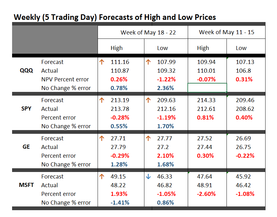
Here is an update on the forecasts from last Monday – forecasts of the high and low of SPY, QQQ, GE, and MSFT.

This table is easy to read, even though it is a little” busy”.

TableMay22

One key is to look at the numbers highlighted in red and blue (click to enlarge).

These are the errors from the week’s forecast based on the NPV algorithm (explained further below) and a No Change forecast.

So if you tried to forecast the high for the week to come, based on nothing more than the high achieved last week – you would be using a No Change model. This is a benchmark in many forecasting discussions, since it is optimal (subject to some qualifications) for a random walk. Of course, the idea stock prices are a random walk came into favor several decades ago, and now gradually is being rejected of modified, based on findings such as those above.

The NPV forecasts are more accurate for this last week than No Change projections 62.5 percent of the time, or in 5 out of the 8 forecasts in the table for the week of May 18-22. Furthermore, in all three cases in which the No Change forecasts were better, the NPV forecast error was roughly comparable in absolute size. On the other hand, there were big relative differences in the absolute size of errors in the situations in which the NPV forecasts proved more accurate, for what that is worth.

The NPV algorithm, by the way, deploys various price ratios (nearby prices) and their transformations as predictors. Originally, the approach focused on ratios of the opening price in a period and the high or low prices in the previous period. The word “new” indicates a generalization has been made from this original specification.

Ridge Regression

I have been struggling with Visual Basic and various matrix programming code for ridge regression with the NPV specifications.

Using cross validation of the λ parameter, ridge regression can improve forecast accuracy on the order of 5 to 10 percent. For forecasts of the low prices, this brings forecast errors closer to acceptable error ranges.

Having shown this, however, I am now obligated to deploy ridge regression in several of the forecasts I provide for a week or perhaps a month ahead.

This requires additional programming to be convenient and transparent to validation.

So, I plan to work on that this coming week, delaying other tables with weekly or maybe monthly forecasts for a week or so.

I will post further during the coming week, however, on the work of Andrew Lo (MIT Financial Engineering Center) and high frequency data sources in business forecasts.

Probable Basis of Success of NPV Forecasts

Suppose you are an observer of a market in which securities are traded. Initially, tests show strong evidence stock prices in this market follow random walk processes.

Then, someone comes along with a theory that certain price ratios provide a guide to when stock prices will move higher.

Furthermore, by accident, that configuration of price ratios occurs and is associated with higher prices at some date, or maybe a couple dates in succession.

Subsequently, whenever price ratios fall into this configuration, traders pile into a stock, anticipating its price will rise during the next trading day or trading period.

Question – isn’t this entirely plausible, and would it not be an example of a self-confirming prediction?

I have a draft paper pulling together evidence for this, and have shared some findings in previous posts. For example, take a look at the weird mirror symmetry of the forecast errors for the high and low.

And, I suspect, the absence or ambivalence of this underlying dynamic is why closing prices are harder to predict than period high or low prices of a stock. If I tell you the closing price will be higher, you do not necessarily buy the stock. Instead, you might sell it, since the next morning opening prices could jump down. Or there are other possibilities.

Of course, there are all kinds of systems traders employ to decide whether to buy or sell a stock, so you have to cast your net pretty widely to capture effects of the main methods.

Long Term Versus Short Term

I am getting mixed results about extending the NPV approach to longer forecast horizons – like a quarter or a year or more.

Essentially, it looks to me as if the No Change model becomes harder and harder to beat over longer forecast horizons – although there may be long run persistence in returns or other features that I see  other researchers (such as Andrew Lo) have noted.

Weekly BusinessForecastBlog Stock Price Forecasts – QQQ, SPY, GE

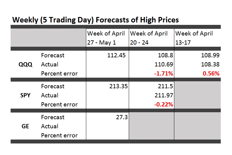
Here are forecasts of the weekly high price for three securities. These include intensely traded exchange traded funds (ETF’s) and a blue chip stock – QQQ, SPY, and GE.

TableA27

The table also shows the track record so far.

All the numbers not explicitly indicated as percents are in US dollars.

These forecasts come with disclaimers. They are presented purely for scientific and informational purposes. This blog takes no responsibility for any investment gains or losses that might be linked with these forecasts. Invest at your own risk.

So having said that, some implications and background information.

First of all, it looks like it’s off to the races for the market as a whole this week, although possibly not for GE. The highs for the ETF’s all show solid gains.

Note, too, that these are forecasts of the high price which will be reached over the next five trading days, Monday through Friday of this week.

Key features of the method are now available in a white paper published under the auspices of the University of Munich – Predictability of the daily high and low of the S&P 500 index. This research shows that the so-called proximity variables achieve higher accuracies in predicting the daily high and low prices for the S&P 500 than do benchmark approaches, such as the no-change forecast and forecasts from an autoregressive model.

Again, caution is advised in making direct application of the methods in the white paper to the current problem –forecasting the high for a five day trading period. There have been many modifications.

That’s, of course, one reason for the public announcements of forecasts from the NPV (new proximity variable) model.

Go real-time, I’ve been advised. It makes the best case, or at least exposes the results to the light of day.

Based on backtesting, I expect forecasts for GE to be less accurate than those for QQQ and SPY. In terms of mean absolute percent error (MAPE), we are talking around 1% for QQQ and SPY and, maybe, 1.7% for GE.

The most reliable element of these forecasts are the indicated directions of change from the previous period highs.

Features and Implications

There are other several other features which are reliably predicted by the NPV models. For example, forecasts for the low price or even closing prices on Friday can be added – although closing prices are less reliable. Obviously, too, volatility metrics are implied by predictions of the high and low prices.

These five-trading day forecasts parallel the results for daily periods documented in the above-cited white paper. That is, the NPV forecast accuracy for these securities in each case beats “no-change” and autoregressive model forecasts.

Focusing on stock market forecasts has “kept me out of trouble” recently. I’m focused on quantitative modeling, and am not paying a lot of attention to global developments – such as the ever- impending Greek default or, possibly, exit from the euro. Other juicy topics include signs of slowing in the global economy, and the impact of armed conflict on the Arabian Peninsula on the global price of oil. These are great topics, but beyond hearsay or personal critique, it is hard to pin things down just now.

So, indeed, I may miss some huge external event which tips this frothy stock market into reverse – but, at the same time, I assure you, once a turning point from some external disaster takes place, the NPV models should do a good job of predicting the extent and duration of such a decline.

On a more optimistic note, my research shows the horizons for which the NPV approach applies and does a better job than the benchmark models. I have, for example, produced backtests for quarterly SPY data, demonstrating continuing superiority of the NPV method.

My guess – and I would be interested in validating this – is that the NPV approach connects with dominant trader practice. Maybe stock market prices are, in some sense, a random walk. But the reactions of traders to daily price movements create short term order out of randomness. And this order can emerge and persist for relatively long periods. And, not only that, but the NPV approach is linked with self-reinforcing tendencies, so that awareness may just make predicted effects more pronounced. That is, if I tell you the high price of a security is going up over the coming period, your natural reaction is to buy in – thus reinforcing the prediction. And the prediction is not just public relations stunt or fluff. The first prediction is algorithmic, rather than wishful and manipulative. Thus, the direction of change is more predictable than the precise extent of price change.

In any case, we will see over coming weeks how well these models do.