Tag Archives: stock market forecasts

I often present at confabs where there are engineers with management or executive portfolios. You start the slides, but, beforehand, prepare for the tough question. Make sure the numbers in the tables add up and that round-off errors or simple typos do not creep in to mess things up.

To carry this on a bit, I recall a Hewlett Packard VP whose preoccupation during meetings was to fiddle with their calculator – which dates the story a little. In any case, the only thing that really interested them was to point out mistakes in the arithmetic. The idea is apparently that if you cannot do addition, why should anyone believe your more complex claims?

I’m bending this around to the theory of efficient markets and rational expectations, by the way.

And I’m playing the role of the engineer.

Rational Expectations

The theory of rational expectations dates at least to the work of Muth in the 1960’s, and is coupled with “efficient markets.”

Lim and Brooks explain market efficiency in – The Evolution of Stock Market Efficiency Over Time: A Survey of the Empirical Literature

The term ‘market efficiency’, formalized in the seminal review of Fama (1970), is generally referred to as the informational efficiency of financial markets which emphasizes the role of information in setting prices.. More specifically, the efficient markets hypothesis (EMH) defines an efficient market as one in which new information is quickly and correctly reflected in its current security price… the weak-form version….asserts that security prices fully reflect all information contained in the past price history of the market.

Lim and Brooks focus, among other things, on statistical tests for random walks in financial time series, noting this type of research is giving way to approaches highlighting adaptive expectations.

Proof US Stock Markets Are Not Efficient (or Maybe That HFT Saves the Concept)

I like to read mathematically grounded research, so I have looked a lot of the papers purporting to show that the hypothesis that stock prices are random walks cannot be rejected statistically.

But really there is a simple constructive proof that this literature is almost certainly wrong.

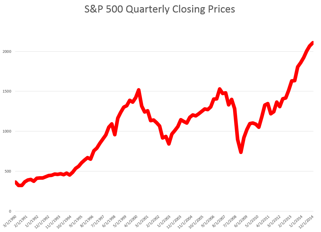
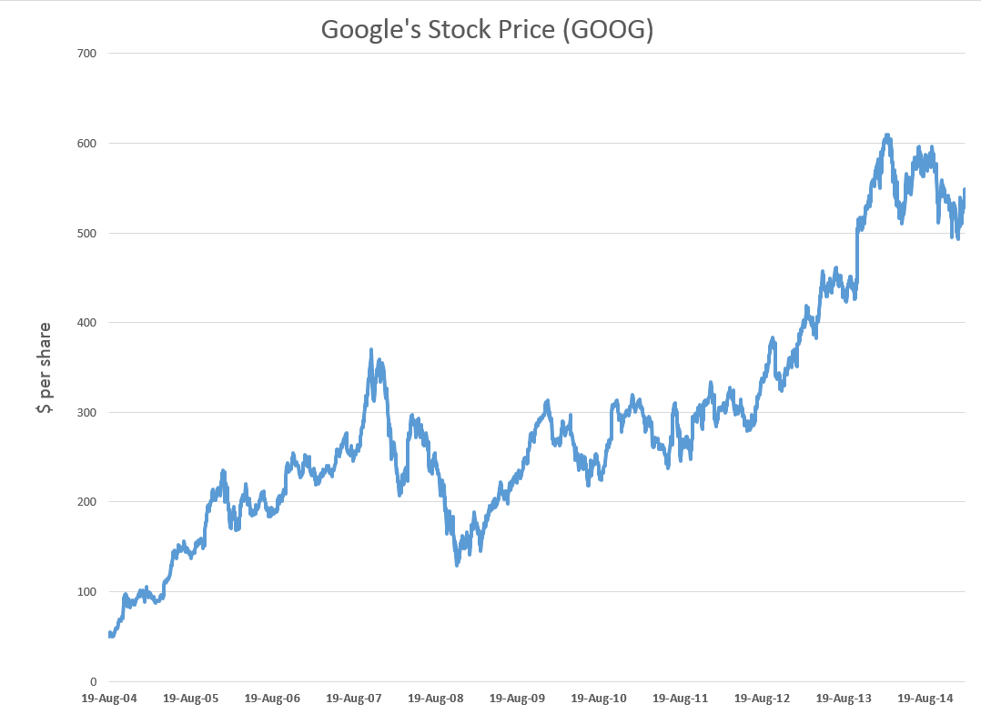
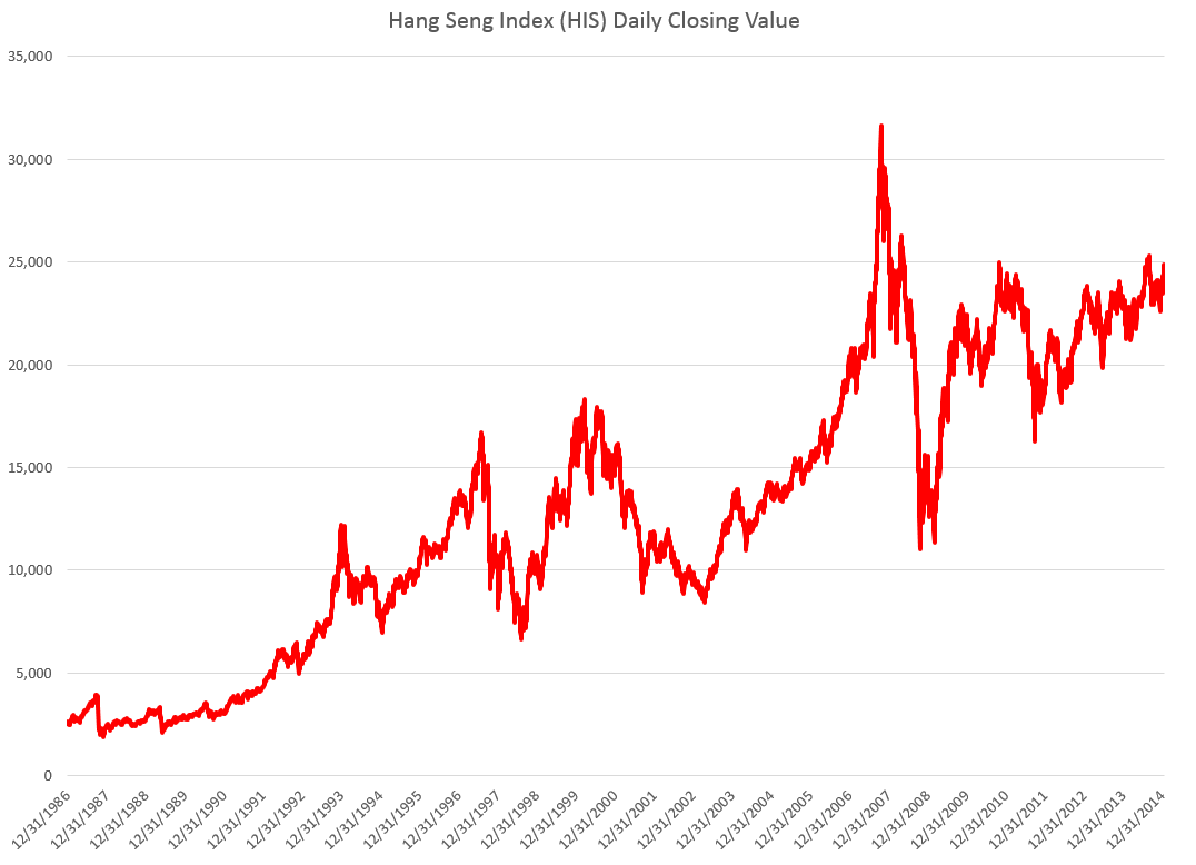
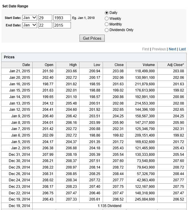
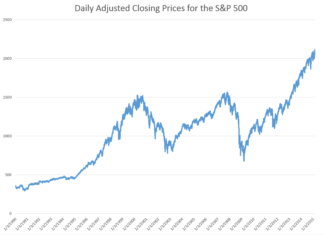
STEP 1: Grab the data. Download daily adjusted closing prices for the S&P 500 from some free site (e,g, Yahoo Finance). I did this again recently, collecting data back to 1990. Adjusted closing prices, of course, are based on closing prices for the trading day, adjusted for dividends and stock splits. Oh yeah, you may have to resort the data from oldest to newest, since a lot of sites present the newest data on top, originally.

Here’s a graph of the data, which should be very familiar by now.

STEP 2: Create the relevant data structure. In the same spreadsheet, compute the trading-day-over-treading day growth in the adjusted closing price (ACP). Then, side-by-side with this growth rate of the ACP, create another series which, except for the first value, maps the growth in ACP for the previous trading day onto the growth of the ACP for any particular day. That gives you two columns of new data.

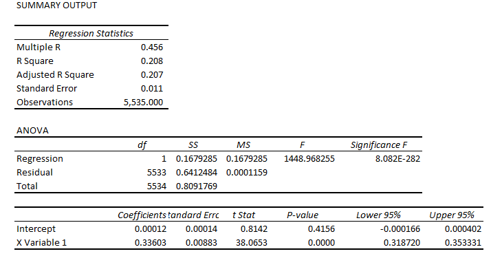
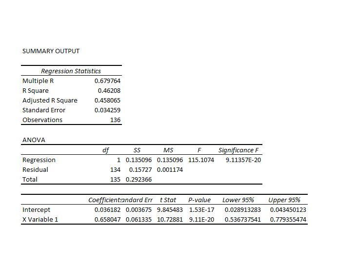
STEP 3: Run adaptive regressions. Most spreadsheet programs include an ordinary least squares (OLS) regression routine. Certainly, Excel does. In any case, you want to setup up a regression to predict the growth in the ACP, based on one trading lags in the growth of the ACP.

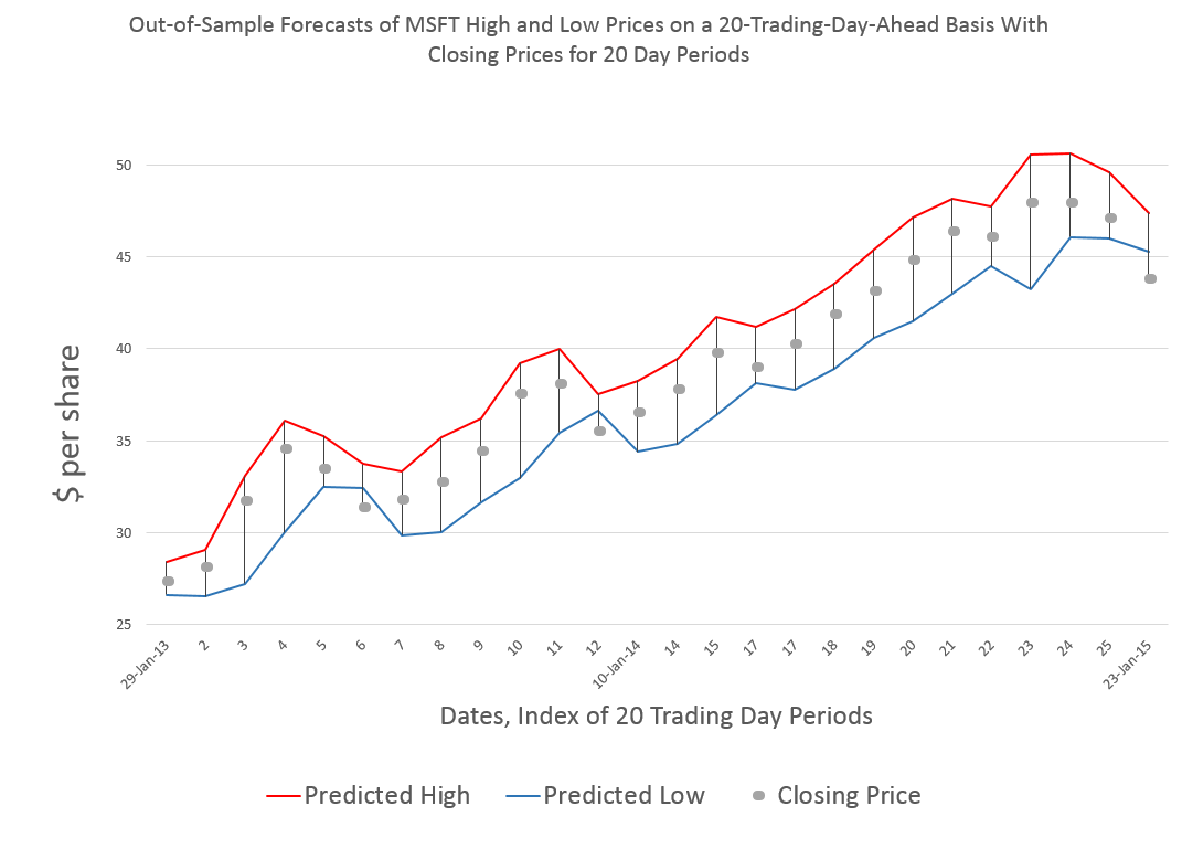
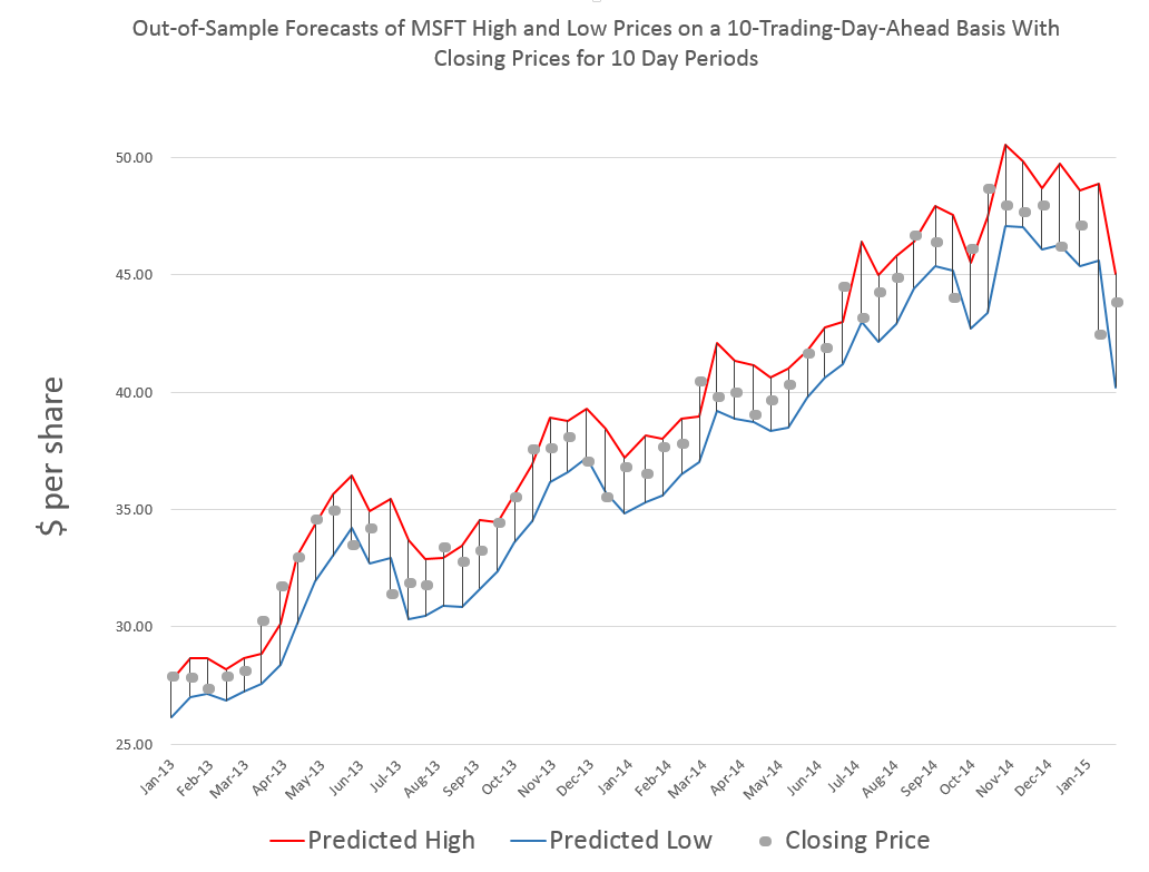
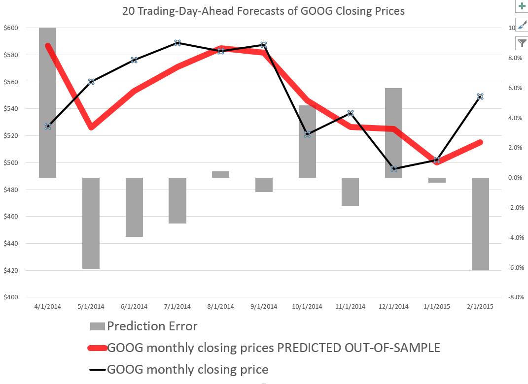
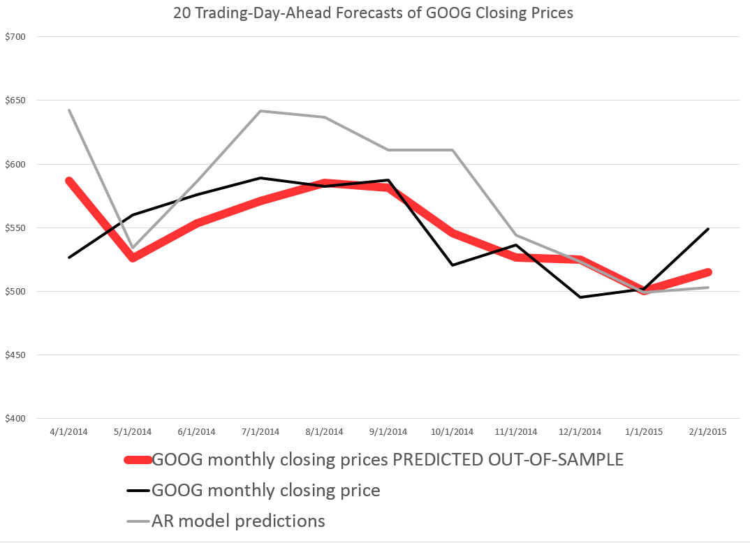
I did this, initially, to predict the growth in ACP for January 3, 2000, based on data extending back to January 3, 1990 – a total of 2528 trading days. Then, I estimated regressions going down for later dates with the same size time window of 2528 trading days.

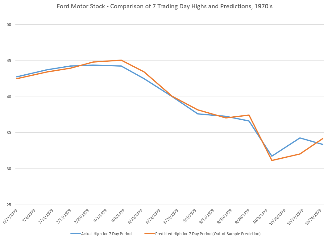
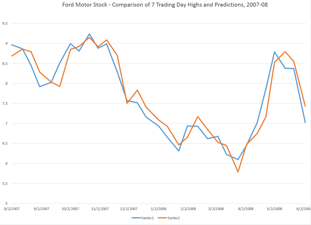
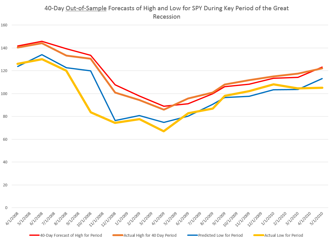
The resulting “predictions” for the growth in ACP are out-of-sample, in the sense that each prediction stands outside the sample of historic data used to develop the regression parameters used to forecast it.

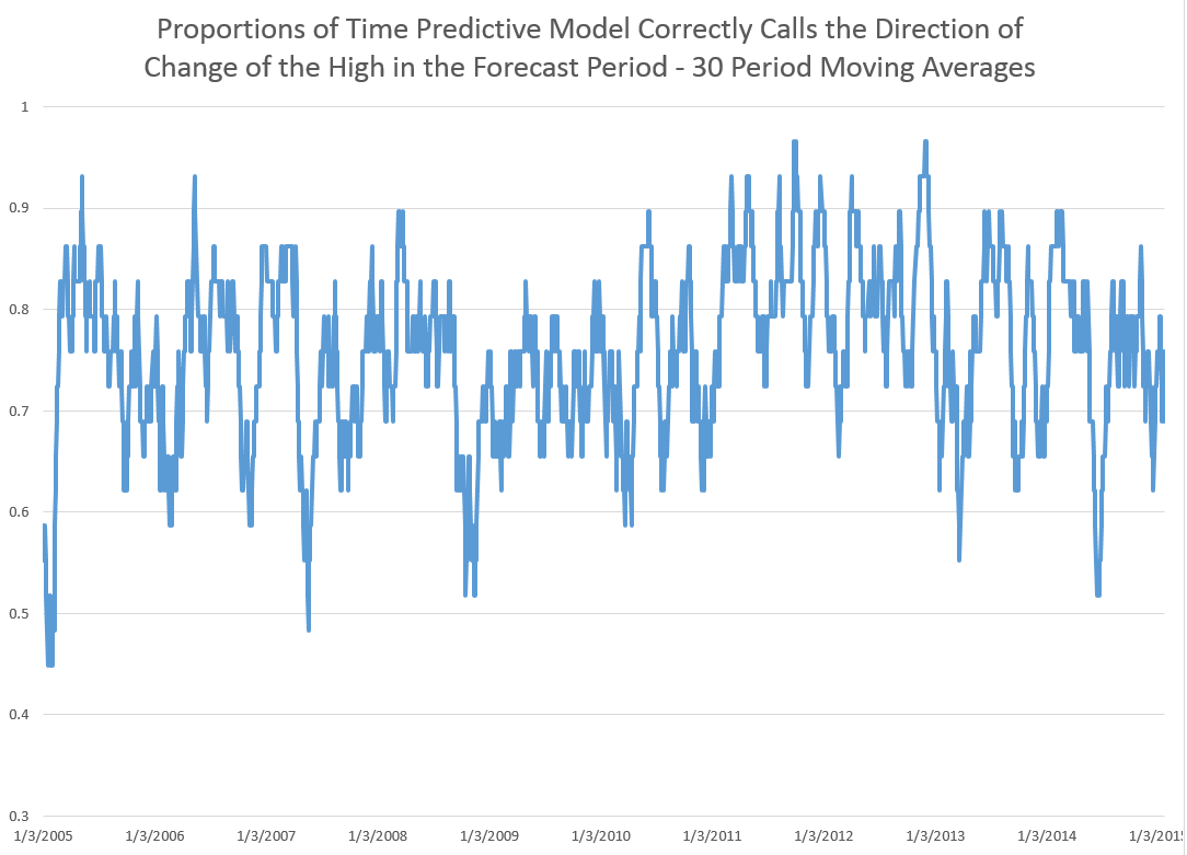
It needs to be said that these predictions for the growth of the adjusted closing price (ACP) are marginal, correctly predicting the sign of the ACP only about 53 percent of the time.

An interesting question, though, is whether these just barely predictive forecasts can be deployed in a successful trading model. Would a trading algorithm based on this autoregressive relationship beat the proverbial “buy-and-hold?”

So, for example, suppose we imagine that we can trade at closing each trading day, close enough to the actual closing prices.

Then, you get something like this, if you invest $100,000 at the beginning of 2000, and trade through last week. If the predicted growth in the ACP is positive, you buy at the previous day’s close. If not, you sell at the previous day’s close. For the Buy-and-Hold portfolio, you just invest the $100,000 January 3, 2000, and travel to Tahiti for 15 years or so.

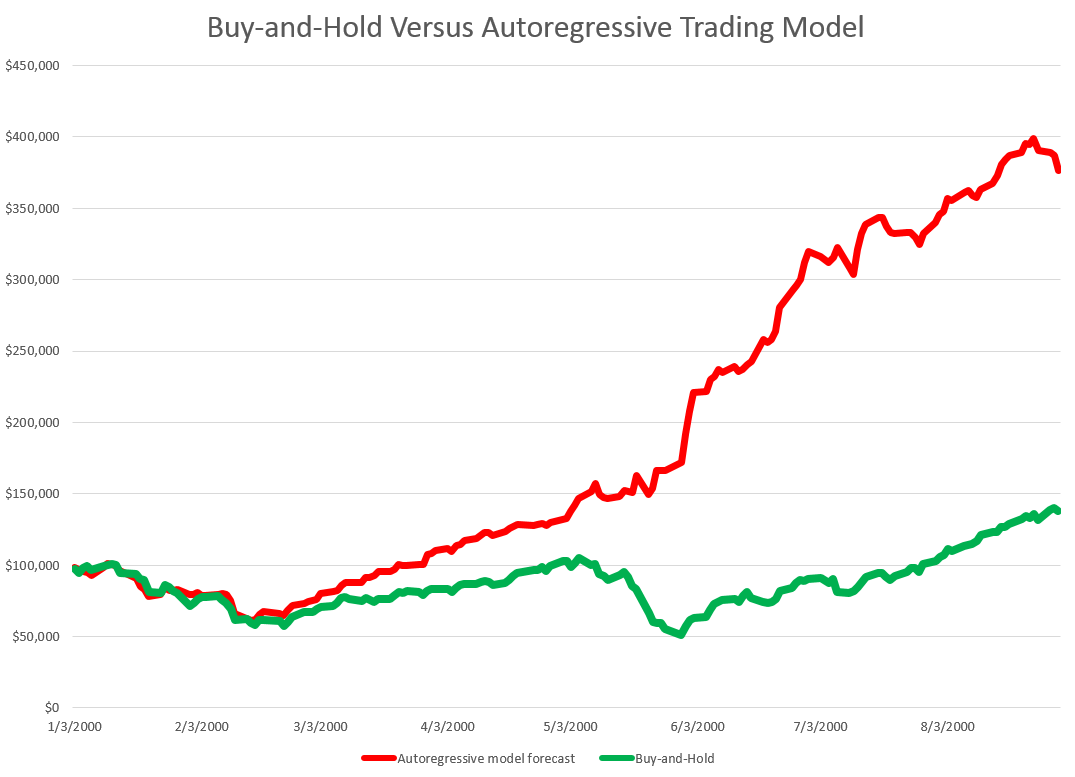
So, as should be no surprise, the Buy-and-Hold strategy results in replicating the S&P 500 Index on a $100,000 base.

The trading strategy based on the simple first order autoregressive model, on the other hand, achieves more than twice these cumulative earnings.

Now I suppose you could say that all this was an accident, or that it was purely a matter of chance, distributed over more than 3,810 trading days. But I doubt it. After all, this trading interval 2000-2015 includes the worst economic crisis since before World War II.

Or you might claim that the profits from the simple AR trading strategy would be eaten up by transactions fees and taxes. On this point, there were 1,774 trades, for an average of $163 per trade. So, worst case, if trading costs $10 a transaction, and there is a tax rate of 40 percent, that leaves $156K over these 14-15 years in terms of take-away profit, or about $10,000 a year.

Where This May Go Wrong

This does sound like a paen to stock market investing – even “day-trading.”

What could go wrong?

Well, I assume here, of course, that exchange traded funds (ETF’s) tracking the S&P 500 can be bought and sold with the same tactics, as outlined here.

Beyond that, I don’t have access to the data currently (although I will soon), but I suspect high frequency trading (HFT) may stand in the way of realizing this marvelous investing strategy.

So remember you have to trade some small instant before market closing to implement this trading strategy. But that means you get into the turf of the high frequency traders. And, as previous posts here observe, all kinds of unusual things can happen in a blink of an eye, faster than any human response time.

So – a conjecture. I think that the choicest situations from the standpoint of this more or less macro interday perspective, may be precisely the places where you see huge spikes in the volume of HFT. This is a proposition that can be tested.

I also think something like this has to be appealed to in order to save the efficient markets hypothesis, or rational expectations. But in this case, it is not the rational expectations of human subjects, but the presumed rationality of algorithms and robots, as it were, which may be driving the market, when push comes to shove.

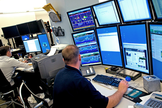
Top picture from CommSmart Global.

forecasting over different forecast horizons, M-competition, stock market forecasts

Scalability of the Pvar Stock Market Forecasting Approach

February 26, 2015 Clive Jones 1 Comment

Ok, I am documenting and extending a method of forecasting stock market prices based on what I call Pvar models. Here Pvar stands for “proximity variable” – or, more specifically, variables based on the spread or difference between the opening price of a stock, ETF, or index, and the high or low of the previous period. These periods can be days, groups of days, weeks, months, and so forth.

I share features of these models and some representative output on this blog.

And, of course, I continue to have wider interests in forecasting controversies, issues, methods, as well as the global economy.

But for now, I’ve got hold of something, and since I appreciate your visits and comments, let’s talk about “scalability.”

Forecast Error and Data Frequency

Years ago, when I first heard of the M-competition (probably later than for some), I was intrigued by reports of how forecast error blows up “three or four periods in the forecast horizon,” almost no matter what the data frequency. So, if you develop a forecast model with monthly data, forecast error starts to explode three or four months into the forecast horizon. If you use quarterly data, you can push the error boundary out three or four quarters, and so forth.

I have not seen mention of this result so much recently, so my memory may be playing tricks.

But the basic concept seems sound. There is irreducible noise in data and in modeling. So whatever data frequency you are analyzing, it makes sense that forecast errors will start to balloon more or less at the same point in the forecast horizon – in terms of intervals of the data frequency you are analyzing.

Well, this concept seems emergent in forecasts of stock market prices, when I apply the analysis based on these proximity variables.

Prediction of Highs and Lows of Microsoft (MSFT) Stock at Different Data Frequencies

What I have discovered is that in order to predict over longer forecast horizons, when it comes to stock prices, it is necessary to look back over longer historical periods.

Here are some examples of scalability in forecasts of the high and low of MSFT.

Forecasting 20 trading days ahead, you get this type of chart for recent 20-day-periods.

One of the important things to note is that these are out-of-sample forecasts, and that, generally, they encapsulate the actual closing prices for these 20 trading day periods.

Here is a comparable chart for 10 trading days.

Same data, forecasts also are out-of-sample, and, of course, there are more closing prices to chart, too.

Finally, here is a very busy chart with forecasts by trading day.

Now there are several key points to take away from these charts.

First, the predictions of MSFT high and low prices for these periods are developed by similar forecast models, at least with regard to the specification of explanatory variables. Also, the Pvar method works for specific stocks, as well as for stock market indexes and ETF’s that might track them.

However, and this is another key point, the definitions of these variables shift with the periods being considered.

So the high for MSFT by trading day is certainly different from the MSFT high over groups of 20 trading days, and so forth.

In any case, there is remarkable scalability with Pvar models, all of which suggests they capture some of the interplay between long and shorter term trading.

While I am handing out conjectures, here is another one.

I think it will be possible to conduct a “causal analysis” to show that the Pvar variables reflect or capture trader actions, and that these actions tend to drive the market.

ARIMA models, autoregressive model, financial forecasting, stock market forecasts

Pvar Models for Forecasting Stock Prices

February 25, 2015 Clive Jones

When I began this blog three years ago, I wanted to deepen my understanding of technique – especially stuff growing up alongside Big Data and machine learning.

I also was encouraged by Malcolm Gladwell’s 10,000 hour idea – finding it credible from past study of mathematical topics. So maybe my performance as a forecaster would improve by studying everything about the subject.

Little did I suspect I would myself stumble on a major forecasting discovery.

But, as I am wont to quote these days, even a blind pig uncovers a truffle from time to time.

Forecasting Stock Prices

My discovery pertains to forecasting stock prices.

Basically, I have stumbled on a method of developing much more accurate forecasts of high and low stock prices, given the opening price in a period. These periods can be days, groups of days, weeks, months, and, based on what I present here – quarters.

Additionally, I have discovered a way to translate these results into much more accurate forecasts of closing prices over long forecast horizons.

I would share the full details, except I need some official acknowledgement for my work (in process) and, of course, my procedures lead to profits, so I hope to recover some of what I have invested in this research.

Having struggled through a maze of ways of doing this, however, I feel comfortable sharing a key feature of my approach – which is that it is based on the spreads between opening prices and the high and low of previous periods. Hence, I call these “Pvar models” for proximity variable models.

There is really nothing in the literature like this, so far as I am able to determine – although the discussion of 52 week high investing captures some of the spirit.

S&P 500 Quarterly Forecasts

Let’s look an example – forecasting quarterly closing prices for the S&P 500, shown in this chart.

We are all familiar with this series. And I think most of us are worried that after the current runup, there may be another major correction.

In any case, this graph compares out-of-sample forecasts of ARIMA(1,1,0) and Pvar models. The ARIMA forecasts are estimated by the off-the-shelf automatic forecast program Forecast Pro. The Pvar models are estimated by ordinary least squares (OLS) regression, using Matlab and Excel spreadsheets.

The solid red line shows the movement of the S&P 500 from 2005 to just recently. Of course, the big dip in 2008 stands out.

The blue line charts out-of-sample forecasts of the Pvar model, which are from visual inspection, clearly superior to the ARIMA forecasts, in orange.

And note the meaning of “out-of-sample” here. Parameters of the Pvar and ARIMA models are estimated over historic data which do not include the prices in the period being forecast. So the results are strictly comparable with applying these models today and checking their performance over the next three months.

The following bar chart shows the forecast errors of the Pvar and ARIMA forecasts.

Thus, the Pvar model forecasts are not always more accurate than ARIMA forecasts, but clearly do significantly better at major turning points, like the 2008 recession.

The mean absolute percent errors (MAPE) for the two approaches are 7.6 and 10.2 percent, respectively.

This comparison is intriguing, since Forecast Pro automatically selected an ARIMA(1,1,0) model in each instance of its application to this series. This involves autoregressions on differences of a time series, to some extent challenging the received wisdom that stock prices are random walks right there. But Pvar poses an even more significant challenge to versions of the efficient market hypothesis, since Pvar models pull variables from the time series to predict the time series – something you are really not supposed to be able to do, if markets are, as it were, “efficient.” Furthermore, this price predictability is persistent, and not just a fluke of some special period of market history.

I will have further comments on the scalability of this approach soon. Stay tuned.

autoregressive model, financial forecasts, stock market forecasts

Forecasting Google’s Stock Price (GOOG) On 20-Trading-Day Horizons

February 16, 2015 Clive Jones

Google’s stock price (GOOG) is relatively volatile, as the following chart shows.

So it’s interesting that a stock market forecasting algorithm can produce the following 20 Trading-Day-Ahead forecasts for GOOG, for the recent period.

The forecasts in the above chart, as are those mentioned subsequently, are out-of-sample predictions. That is, the parameters of the forecast model – which I call the PVar model – are estimated over one set of historic prices. Then, the forecasts from PVar are generated with values for the explanatory variables that are “outside” or not the same as this historic data.

How good are these forecasts and how are they developed?

Well, generally forecasting algorithms are compared with benchmarks, such as an autoregressive model or a “no-change” forecast.

So I constructed an autoregressive (AR) model for the Google closing prices, sampled at 20 day frequencies. This model has ten lagged versions of the closing price series, so I do not just rely here on first order autocorrelations.

Here is a comparison of the 20 trading-day-ahead predictions of this AR model, the above “proximity variable” (PVar) model which I take credit for, and the actual closing prices.

As you can see, the AR model is worse in comparison to the PVar model, although they share some values at the end of the forecast series.

The mean absolute percent errors (MAPE) of the AR model for a period more extended than shown in the graph is 7.0, compared with 5.1 for PVar. This comparison is calculated over data from 4/20/2011.

So how do I do it?

Well, since these models show so much promise, it makes sense to keep working on them, making improvements. However, previous posts here give broad hints, indeed pretty well laying out the framework, at least on an introductory basis.

Essentially, I move from predicting highs and lows to predicting closing prices.

To predict highs and lows, my post “further research” states

Now, the predictive models for the daily high and low stock price are formulated, as before, keying off the opening price in each trading day. One of the key relationships is the proximity of the daily opening price to the previous period high. The other key relationship is the proximity of the daily opening price to the previous period low. Ordinary least squares (OLS) regression models can be developed which do a good job of predicting the direction of change of the daily high and low, based on knowledge of the opening price for the day.

Other posts present actual regression models, although these are definitely prototypes, based on what I know now.

Why Does This Work?

I’ll bet this works because investors often follow simple rules such as “buy when the opening price is sufficiently greater than the previous period high” or “sell, if the opening price is sufficiently lower than the previous period low.”

I have assembled evidence, based on time variation in the predictive coefficients of the PVar variables, which I probably will put out here sometime.

But the point is that momentum trading is a major part of stock market activity, not only in the United States, but globally. There’s even research claiming to show that momentum traders do better than others, although that’s controversial.

This means that the daily price record for a stock, the opening, high, low, and closing prices, encode information that investors are likely to draw upon over different investing horizons.

I’m pleased these insights open up many researchable questions. I predict all this will lead to wholly new generations of models in stock market analysis. And my guess, and so far it is largely just that, is that these models may prove more durable than many insights into patterns of stock market prices – due to a sort of self-confirming aspect.

automatic forecasting software, predictive analytics, stock trading algorithms

High Frequency Trading – 2

February 4, 2015 Clive Jones

High Frequency Trading (HFT) occurs faster than human response times – often quoted as 750 milliseconds. It is machine or algorithmic trading, as Sean Gourley’s “High Frequency Trading and the New Algorithmic Ecosystem” highlights.

This is a useful introductory video.

It mentions Fixnetix’s field programmable array chip and new undersea cables designed to shave milliseconds off trading speeds from Europe to the US and elsewhere.

Also, Gourley refers to dark pool pinging, which tries to determine the state of large institutional orders by “sniffing them out” and using this knowledge to make (almost) risk-free arbitrage by trading on different exchanges in milliseconds or faster. Institutional investors using slower and not-so-smart algorithms lose.

Other HFT tractics include “quote stuffing”, “smoking”, and “spoofing.” Of these, stuffing may be the most damaging. It limits access of slower traders by submitting large numbers of orders and then canceling them very quickly. This leads to order congestion, which may create technical trouble and lagging quotes.

Smoking and spoofing strategies, on the other hand, try to manipulate other traders to participate in trading at unfavorable moments, such as just before the arrival of relevant news.

Here are some more useful links on this important development and the technological arms race that has unfolded around it.

Financial black swans driven by ultrafast machine ecology Key research on ultrafast black swan events

Nanosecond Trading Could Make Markets Go Haywire Excellent Wired article

High-Frequency Trading and Price Discovery

Defense of HFT on basis that HFTs’ trade (buy or sell) in the direction of permanent price changes and against transitory pricing errors creates benefits which outweigh adverse selection of HFT liquidity supplying (non-marketable) limit orders.

The Good, the Bad, and the Ugly of Automated High-Frequency Trading tries to strike a balance, but tilts toward a critique

Has HFT seen its heyday? I read at one and the same time I read at one and the same time that HFT profits per trade are dropping, that some High Frequency Trading companies report lower profits or are shutting their doors, but that 70 percent of the trades on the New York Stock Exchange are the result of high frequency trading.

My guess is that HFT is a force to be dealt with, and if financial regulators are put under restraint by the new US Congress, we may see exotic new forms flourishing in this area.

Big Data, stock market forecasts, stock trading algorithms

High Frequency Trading and the Efficient Market Hypothesis

January 29, 2015 Clive Jones 2 Comments

Working on a white paper about my recent findings, I stumbled on more confirmation of the decoupling of predictability and profitability in the market – the culprit being high frequency trading (HFT).

It makes a good story.

So I am looking for high quality stock data and came across the CalTech Quantitative Finance Group market data guide. They tout QuantQuote, which does look attractive, and was cited as the data source for – How And Why Kraft Surged 29% In 19 Seconds – on Seeking Alpha.

In early October 2012 (10/3/2012), shares of Kraft Foods Group, Inc surged to a high of $58.54 after opening at $45.36, and all in just 19.93 seconds. The Seeking Alpha post notes special circumstances, such as spinoff of Kraft Foods Group, Inc. (KRFT) from Modelez International, Inc., and addition of KRFT to the S&P500. Funds and ETF’s tracking the S&P500 then needed to hold KRFT, boosting prospects for KRFT’s price.

For 17 seconds and 229 milliseconds after opening October 3, 2012, the following situation, shown in the QuantQuote table, unfolded.

Times are given in milliseconds past midnight with the open at 34200000.

There is lots of information in this table – KRFT was not shortable (see the X in the Short Status column), and some trades were executed for dark pools of money, signified by the D in the Exch column.

In any case, things spin out of control a few milliseconds later, in ways and for reasons illustrated with further QuantQuote screen shots.

The moral –

So how do traders compete in a marketplace full of computers? The answer, ironically enough, is to not compete. Unless you are prepared to pay for a low latency feed and write software to react to market movements on the millisecond timescale, you simply will not win. As aptly shown by the QuantQuote tick data…, the required reaction time is on the order of 10 milliseconds. You could be the fastest human trader in the world chasing that spike, but 100% of the time, the computer will beat you to it.

CNN’s Watch high-speed trading in action is a good companion piece to the Seeking Alpha post.

HFT trading has grown by leaps and bounds, but estimates vary – partly because NASDAQ provides the only Datasets to academic researchers that directly classify HFT activity in U.S. equities. Even these do not provide complete coverage, excluding firms that also act as brokers for customers.

Still, the Security and Exchange Commission (SEC) 2014 Literature Review cites research showing that HFT accounted for about 70 percent of NASDAQ trades by dollar volume.

And associated with HFT are shorter holding times for stocks, now reputed to be as low as 22 seconds, although Barry Ritholz contests this sort of estimate.

Felix Salmon provides a list of the “evils” of HFT, suggesting a small transactions tax might mitigate many of these,

But my basic point is that the efficient market hypothesis (EMH) has been warped by technology.

I am leaning to the view that the stock market is predictable in broad outline.

But this predictability does not guarantee profitability. It really depends on how you handle entering the market to take or close out a position.

As Michael Lewis shows in Flash Boys, HFT can trump traders’ ability to make a profit

financial forecasting, forecasting research, predicting turning points, stock market forecasts

Stock Market Predictability

January 27, 2015 Clive Jones

The research findings in recent posts here suggest that, in broad outline, the stock market is predictable.

This is one of the most intensively researched areas of financial econometrics.

There certainly is no shortage of studies claiming to forecast stock prices. See for example, Atsalakis, G., and K. Valavanis. “Surveying stock market forecasting techniques-part i: Conventional methods.” Journal of Computational Optimization in Economics and Finance 2.1 (2010): 45-92.

But the field is dominated by decades-long controversy over the efficient market hypothesis (EMH).

I’ve been reading Lim and Brooks outstanding survey article – The Evolution of Stock Market Efficiency Over Time: A Survey of the Empirical Literature.

They highlight two types of studies focusing on the validity of a weak form of the EMH which asserts that security prices fully reflect all information contained in the past price history of the market…

The first strand of studies, which is the focus of our survey, tests the predictability of security returns on the basis of past price changes. More specifically, previous studies in this sub-category employ a wide array of statistical tests to detect different types of deviations from a random walk in financial time series, such as linear serial correlations, unit root, low-dimensional chaos, nonlinear serial dependence and long memory. The second group of studies examines the profitability of trading strategies based on past returns, such as technical trading rules (see the survey paper by Park and Irwin, 2007), momentum and contrarian strategies (see references cited in Chou et al., 2007).

Another line, related to this second branch of research tests.. return predictability using other variables such as the dividend–price ratio, earnings–price ratio, book-to-market ratio and various measures of the interest rates.

Lim and Brooks note the tests for the semi-strong-form and strong-form EMH are renamed as event studies and tests for private information, respectively.

So bottom line – maybe your forecasting model predicts stock prices or rates of return over certain periods, but the real issue is whether it makes money. As Granger writes much earlier, mere forecastability is not enough.

I certainly respect this criterion, and recognize it is challenging. It may be possible to trade on the models of high and low stock prices over periods such I have been discussing, but I can also show you situations in which the irreducibly stochastic elements in the predictions can lead to losses. And avoiding these losses puts you into the field of higher frequency trading, where “all bets are off,” since there is so much that is not known about how that really works, particularly for individual investors.

My primary purpose, however, in pursuing these types of models is originally not so much for trading (although that is seductive), but to explore new ways of forecasting turning points in economic time series. Confronted with the dismal record of macroeconomic forecasters, for example, one can see that predicting turning points is a truly fundamental problem. And this is true, I hardly need to add, for practical business forecasts. Your sales may do well – and exponential smoothing models may suffice – until the next phase of the business cycle, and so forth.

So I am amazed by the robustness of the turning point predictions from the longer (30 trading days, 40 days, etc.) groupings.

I just have never myself developed or probably even seen an example of predicting turning points as clearly as the one I presented in the previous post relating to the Hong Kong Hang Seng Index.

A Simple Example of Stock Market Predictability

Again, without claims as to whether it will help you make money, I want to close this post today with comments about another area of stock price predictability – perhaps even simpler and more basic than relationships regarding the high and low stock price over various periods.

This is an exercise you can try for yourself in a few minutes, and which leads to remarkable predictive relationships which I do not find easy to identify or track in the existing literature regarding stock market predictability.

First, download the Yahoo Finance historical data for SPY, the ETF mirroring the S&P 500. This gives you a spreadsheet with approximately 5530 trading day values for the open, high, low, close, volume, and adjusted close. Sort from oldest to most recent. Then calculate trading-day over trading-day growth rates, for the opening prices and then the closing prices. Then, set up a data structure associating the opening price growth for day t with the closing price growth for day t-1. In other words, lag the growth in the closing prices.

Then, calculate the OLS regression of growth in lagged closing prices onto the growth in opening prices.

You should get something like,

This is, of course, an Excel package regression output. It indicates that X Variable 1, which is the lagged growth in the closing prices, is highly significant as an explanatory variable, although the intercept or constant is not.

This equation explains about 21 percent of the variation in the growth data for the opening prices.

It also successfully predicts the direction of change of the opening price about 65 percent of the time, or considerably better than chance.

Not only that, but the two and three-period growth in the closing prices are successful predictors of the two and three-period growth in the opening prices.

And it probably is possible to improve the predictive performance of these equations by autocorrelation adjustments.

Comments

Why present the above example? Well, because I want to establish credibility on the point that there are clearly predictable aspects of stock prices, and ones you perhaps have not heard of heretofore.

The finance literature on stock market prediction and properties of stock market returns, not to mention volatility, is some of the most beautiful and complex technical literatures I know of.

But, still, I think new and important relationships can be discovered.

Whether this leads to profit-making is another question. And really, the standards have risen significantly in recent times, with program and high frequency trading possibly snatching profit opportunities from traders at the last microsecond.

So I think the more important point, from a policy standpoint if nothing else, may be whether it is possible to predict turning points – to predict broader movements of stock prices within which high frequency trading may be pushing the boundary.

predicting turning points, regression forecasts, stock market forecasts

Analysis of Highs and Lows of the Hong Kong Hang Seng Index, 1987 to the Present

January 26, 2015 Clive Jones 6 Comments

I have discovered a fundamental feature of stock market prices, relating to prediction of the highs and lows in daily, weekly, monthly, and to other more arbitrary groupings of trading days in consecutive blocks.

What I have found is a degree of predictability previously unimagined with respect to forecasts of the high and low for a range of trading periods, extending from daily to 60 days so far.

Currently, I am writing up this research for journal submission, but I am documenting essential features of my findings on this blog.

A few days ago, I posted about the predictability of daily highs and lows for the SPY exchange traded fund. Subsequent posts highlight the generality of the result for the SPY, and more recently, for stocks such as common stock of the Ford Motor Company.

These posts present various graphs illustrating how well the prediction models for the high and low in periods capture the direction of change of the actual highs and lows. Generally, the models are right about 70 to 80 percent of the time, which is incredible.

Furthermore, since one of my long concerns has been to get better forward perspective on turning points – I am particularly interested in the evidence that these models also do fairly well as predicting turning points.

Finally, it is easy to show that these predictive models for the highs and lows of stocks and stock indices over various periods, furthermore, are not simply creations of modern program trading. The same regularities can be identified in earlier periods before easy access to computational power, in the 1980’s and early 1990’s, for example.

Hong Kong’s Hang Seng Index

Today, I want to reach out and look at international data and present findings for Hong Kong’s Hang Seng Index. I suspect Chinese investors will be interested in these results. Perhaps, releasing this information to such an active community of traders will test my hypothesis that these are self-fulfilling predictions, to a degree, and knowledge of their existence intensifies their predictive power.

A few facts about the Hang Seng Index – The Hang Seng Index (HSI) is a free-float adjusted, capitalization-weighted index of approximately 40 of the larger companies on the Hong Kong exchange. First published in 1969, the HSI, according to Investopedia, covers approximately 65% of the total market capitalization of the Hong Kong Stock Exchange. It is currently maintained by HSI Services Limited, a wholly owned subsidiary of Hang Seng Bank – the largest bank registered and listed in Hong Kong in terms of market capitalization.

For data, I download daily open, high, low, close and other metrics from Yahoo Finance. This data begins with the last day in 1986, continuing to the present.

The Hang Seng is a volatile index, as the following chart illustrates.

Now there are peculiarities about the data on HSI from Yahoo. Trading volumes are zero until 2001, for example, after which time large positive values are to be found in the volume column. Initially, I assume HSI was a pure index and later came to be actually traded in some fashion.

Nevertheless, the same type of predictive models can be developed for the Hang Seng Index, as can be estimated for the SPY and the US stocks.

Again, the key variables in these predictive relationships are the proximity of the period opening price to the previous period high and the previous period low. I estimate regressions with variables constructed from these explanatory variables, mapping them onto growth in period-by-period highs with ordinary least squares (OLS). I find the similar relationships for the Hang Seng in, say, a 30 day periodization as I estimate for the SPY ETF. At the same time there are differences, one of the most notable being the significantly less first order autocorrelation in the Hang Seng regression.

Essentially, higher growth rates for the period-over-previous-period high are predicted whenever the opening price of the current period is greater than the high of the previous period. There are other cases, however, and ultimately the rule is quantitative, taking into account the size of the growth rates for the high as well as these inequality relationships.

Findings

Here is another one of those charts showing the “hit-rate” for predictions of the direction of change of the sign of period-by-period growth rates for the high. In this case, the chart refers to daily trading data. The chart graphs 30 day moving averages of the proportions of time in which the predictive model forecasts the correct sign of the change or growth in the target or independent variable – the growth rate of daily highs (for consecutive trading days). Note that for recent years, the “hit rate” of the predictive model approaches 90 percent of the time, and all these are all out-of-sample predictions.

The relationship for the Hang Seng Index, thus, is powerful. Similarly impressive relationships can be derived to predict the daily lows and their direction of change.

But the result I really like with this data is developed with grouping the daily trading data by 30 day intervals.

If you do this, you develop a tool which apparently is quite capable of predicting turning points in the Hang Seng.

Thus, between April 2005 and August 2012, a 30-day predictive model captures many of the key features of inflection and turning in the Hang Seng High for comparable periods.

Note that the predictive model makes these forecasts of the high for a period out-of-sample. All the relationships are estimated over historical data which do not include the high (or low) being predicted for the coming 30 day period. Only the opening price for the Hang Seng for that period is necessary.

Concluding Thoughts

I do not present the regression results here, but am pleased to share further information for readers responding to the Comments section to this blog (title ” Request for High/Low Model Information”) or who send requests to the following mail address: Clive Jones, PO Box 1009, Boulder, CO 80306 USA.

Top image from Ancient Chinese Fashion

predicting turning points, stock market forecasts, stock trading algorithms

Further Research into Predicting Daily and Other Period High and Low Stock Prices

January 23, 2015 Clive Jones 3 Comments

The Internet is an amazing scientific tool. Communication of results is much faster, although, of course, with, potentially, dreck and misinformation. At the same time, pressures within the academy and Big Science seem to translate into a shocking amount of bogus research being touted. So maybe this free-for-all on the Web is where it’s at, if you are trying to get up to speed on new findings.

So this post today seeks to nail down some further and key points about predicting the high and low of stocks over various periods – conventionally, daily, weekly, and monthly periods, but also, as I have discovered, highs and lows over consecutive blocks of trading days ranging from 1 to 60 days, and probably more.

My recent posts focus on the SPY exchange traded fund, which tracks the S&P 500.

Yesterday, I formulated my general findings as follows:

For every period from daily periods to 60 day periods I have investigated, the high and low prices are “relatively” predictable and the direction of change from period to period is predictable, in backcasting analysis, about 70-80 percent of the time, on average.

In this post, let me show you the same basic relationship for a common stock – Ford Motor stock (F). I also consider data from the 1970’s, as well as recent data, to underline that modern program or high-speed computer-based algorithms have nothing to do with the underlying pattern.

I also show that the predictive model for the high in a period successfully captures turning points in the stock price in the 1970’s and more recently for 2008-2009.

Approach

Yahoo Finance, my free source of daily trading data, has history for Ford Motor stock dating back to June 1, 1972, charted as follows.

Predicting the Direction of Change of the High

As before, these models make correct predictions regarding the directions of change of the high and low about 70 percent of the time.

Here are 30 period moving averages for the 1970’s, showing the proportions of time the predictive model for the daily high is right about the direction of change.

So the underlying relationship definitely holds in this age in which computer modeling of trading was in its infancy.

Here is a similar chart for the first decade of this century.

So whether we are considering the 1970’s or the last ten years, these predictive models do well in forecasting the direction of change of the high in daily (and it turns out other) periods.

Predicting Turning Points

We can make the same type of comparison – between the 1970’s and more recent years – for the capability of the predictive models to forecast turning points in the stock high (or low).

To do this usually requires aggregating the stock data. In the charts below, I aggregate to 7 trading day periods – not quite the same as weekly periods, since weekly segmentation can be short a day and so forth.

So the high which the predictive model focuses on is the high for the coming seven trading days, given the current day opening price.

Here are two charts, one for dates in the 1970’s and the other for a period in the recession of 2008-2009. For each chart I estimate OLS regressions with data predating each forecast of the high, based on blocks of 7 trading days.

These predictions of the high crisply capture most of the important turning and inflection point features.

The application of similar predictive models for the 2008-2009 period is a little choppier, but does nail many of the important swings in the direction of change of the high of Ford Motor stock.

Concluding Thoughts

Well, this relationship between the opening prices and previous period highs and lows is highly predictive of the direction of change of the highs and lows in the current period – which can be a span of time from a day to 60 days in my findings.

These predictive models work for the S&P 500 and for individual stocks, like Ford Motor (and I might add Exxon and Microsoft).

They work in recent time periods and way back in the 1970’s.

And there’s more – for example, one could argue these patterns in the high and low prices are fractal, in the sense they represent “self similarity” at all (really many or a range of) time scales.

This is literally a new and fundamental regularity in stock prices.

Why does this work?

Well, the predictive models are closely related to very simple momentum trading strategies. But I think there is a lot of research to be done here. If you want further detail on any of this, please put your request in the Comments with the heading “Request for High/Low Model Information.”

Top picture from Strategic Monk.

predicting turning points, predictive analytics, regression forecasts, stock market forecasts

Forecasting the S&P 500 – Short and Long Time Horizons

January 22, 2015 Clive Jones

Friends and acquaintances know that I believe I have discovered amazing, deep, and apparently simple predictability in aspects of the daily, weekly, monthly movement of stock prices.

People say – “don’t blog about it, keep it to yourself, and use it to make a million dollars.” That does sound attractive, but I guess I am a data scientist, rather than stock trader. Not only that, but the pattern looks to be self-fulfilling. Generally, the result of traders learning about this pattern should be to reinforce, rather than erase, it. There seems to be no other explanation consistent with its long historical vintage, nor the broadness of its presence. And that is big news to those of us who like to linger in the forecasting zoo.

I am going to share my discovery with you, at least in part, in this blog post.

But first, let me state some ground rules and describe the general tenor of my analysis. I am using OLS regression in spreadsheets at first, to explore the data. I am only interested, really, in models which have significant out-of-sample prediction capabilities. This means I estimate the regression model over a set of historical data and then use that model to predict – in this case the high and low of the SPY exchange traded fund. The predictions (or “retrodictions” or “backcasts”) are for observations on the high and low stock prices for various periods not included in the data used to estimate the model.

Now let’s look at the sort of data I use. The following table is from Yahoo Finance for the SPY. The site allows you to download this data into a spreadsheet, although you have to invert the order of the dating with a sort on the date. Note that all data is for trading days, and when I speak of N-day periods in the following, I mean periods of N trading days.

OK, now let me state my major result.

To give an example of a backcasting analysis, consider this chart from the period of free-fall in markets during 2008-2009, the Great Recession (click to enlarge).

Now note that the indicated lines for the forecasts are not, strictly-speaking, 40-day-ahead forecasts. The forecasts are for the level of the high and low prices of the SPY which will be attained in each period of 40 trading days.

But the point is these rather time-indeterminate forecasts, when graphed alongside the actual highs and lows for the 40 trading day periods in question, are relatively predictive.

More to the point, the forecasts suffice to signal a key turning point in the SPY. Of course, it is simple to relate the high and low of the SPY for a period to relevant measures of the average or closing stock prices.

So seasoned forecasters and students of the markets and economics should know by this example that we are in terra incognita. Forecasting turning points out-of-sample is literally the toughest thing to do in forecasting, and certain with respect to the US stock market.

Many times technical analysts claim to predict turning points, but their results may seem more artistic, involving subtle interpretations of peaks and shoulders, as well as levels of support.

Now I don’t want to dismiss technical analysis, since, indeed, I believe my findings may prove out certain types of typical results in technical analysis. Or at least I can see a way to establish that claim, if things work out empirically.

Forecast of SPY High And Low for the Next Period of 40 Trading Days

What about the coming period of 40 trading days, starting from this morning’s (January 22, 2015) opening price for the SPY – $203.99?

Well, subject to qualifications I will state further on here, my estimates suggest the high for the period will be in the range of $215 and the period low will be around $194. Cents attached to these forecasts would be, of course, largely spurious precision.

In my opinion, these predictions are solid enough to suggest that no stock market crash is in the cards over the next 40 trading days, nor will there be a huge correction. Things look to trade within a range not too distant from the current situation, with some likelihood of higher highs.

It sounds a little like weather forecasting.

The Basic Model

Here is the actual regression output for predicting the 40 trading day high of the SPY.

This is a simpler than many of the models I have developed, since it only relies on one explanatory variable designated X Variable 1 in the Excel regression output. This explanatory variable is the ratio of the current opening price to the previous high for the 40 day trading period, all minus 1.

Let’s call this -1+ O/PH. Instances of -1+ O/PH are generated for data bunched by 40 trading day periods, and put into the regression against the growth in consecutive highs for these 40 day periods.

So what happens is this, apparently.

Everything depends on the opening price. If the high for the previous period equals the opening price, the predicted high for the next 40 day period will be the same as the high for the previous 40 day period.

If the previous high is less than the opening price, the prediction is that the next period high will be higher. Otherwise, the prediction is that the next period high will be lower.

This then looks like a trading rule which even the numerically challenged could follow.

And this sort of relationship is not something that has just emerged with quants and high frequency trading. On the contrary, it is possible to find the same type of rule operating with, say, Exxon’s stock (XOM) in the 1970’s and 1980’s.

But, before jumping to test this out completely, understand that the above regression is, in terms of most of my analysis, partial, missing at least one other important explanatory variable.

Previous posts, which employ similar forecasting models for daily, weekly, and monthly trading periods, show that these models can predict the direction of change of the period highs with about 70 to 80 percent accuracy (See, for example, here).

Provisos and Qualifications

In deploying OLS regression analysis, in Excel spreadsheets no less, I am aware there are many refinements which, logically, might be developed and which may improve forecast accuracy.

One thing I want to stress is that residuals of the OLS regressions on the growth in the period highs generally are not normally distributed. The distribution tends to be very peaked, reminiscent of discussions earlier in this blog of the Laplace distribution for Microsoft stock prices.

There also is first order serial correlation in many of these regressions. And, my software indicates that there could be autocorrelations extending deep into the historical record.

Finally, the regression coefficients may vary over the historical record.

Bottom LIne

I like Robb Hyndman’s often drawn distinction between modeling and reality. Somewhere Hyndman suggests that no model is right.

But this class of models has an extremely logical motivation, and is, as I say, relatively predictive – predictive enough to be useful in a number of contexts.

Momentum traders for years apparently have looked at the opening price and compared it with the highs (and lows) for previous periods – extending 60 days or more into history if not more – and decided whether to trade. If the opening price is greater than the past high, the next high is anticipated to be even higher. On this basis, stock may be purchased. That action tends to reinforce the relationship. So, in some sense, this is a self-fulfilling relationship.

To recapitulate – I can show you iron-clad, incontrovertible evidence that some fairly simple models built on daily trading data produce workable forecasts of the high and low for stock indexes and stocks. These forecasts are available for a variety of time periods, and, apparently, in backcasts can indicate turning points in the market.

As I say, feel free to request further documentation. I am preparing a write-up for a journal, and I think I can find a way to send out versions of this.

You can contact me confidentially via the Comments box below. Leave your email or phone number. Title the Comment “Request for High/Low Model Information” and the webmeister will forward it to me without having your request listed in the side panel of the blog.

Business Forecasting