Category Archives: Bayesian methods

Global Population in 2100

May 20, 2015 Clive Jones

Probabilistic and Bayesian methods suggest global population will reach about 11 billion by 2100. Stabilization, zero population growth, or population declines are not likely to occur in this century.

These projections come from an article in Foresight, which styles itself the International Journal of Applied Forecasting.

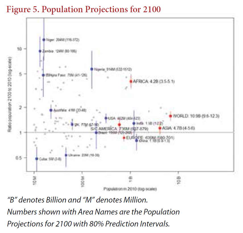
Here’s an exhibit from the article (“The United Nations Probabilistic Population Projections: An Introduction to Demographic Forecasting with Uncertainty”). If you can read through the haze in the reproduction, I found some interesting stuff (click to enlarge). Africa, for example, significantly approaches Asia in population – both with more than 4 billion persons. China is projected to still have more people than India, and the population of Nigeria will be just short of one billion.

The projections are constructed with a cohort component projection method, which projects populations by sex and and five-year age groups based on possible future trajectories of fertility, mortality, and migration.

Traditionally, the UN produced deterministic population projections and point forecasts, supplemented with ranges based on scenarios.

In 2014, however, the United Nations issued its first probabilistic population projections that attempt to quantify the uncertainty of the forecasts.

In the probabilistic method, uncertainty is captured by building a large sample of future trajectories for population size and other demographic metrics. Median outcomes then are used for point forecasts.

A key aspect the methodology is predicting fertility rates by county.

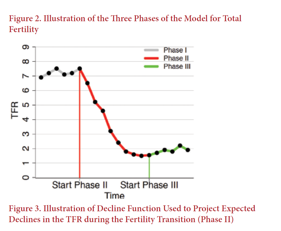
There are three phases to fertility, high fertility Phase I, a phrase involving a steep decline, down to the Phase III – the post-fertility transition.

Most developed countries are in phase III. All countries have completed Phase I.

The article explains, more clearly than I have found heretofore, how probabilistic projections and Bayesian methods can be combined in population forecasting. Really one of the best, short treatments of the topic I have found.

Bayesian methods, data science, machine learning, natural language processing, predictive analytics, Uncategorized

Video Friday – Andrew Ng’s Machine Learning Course

July 18, 2014 Clive Jones

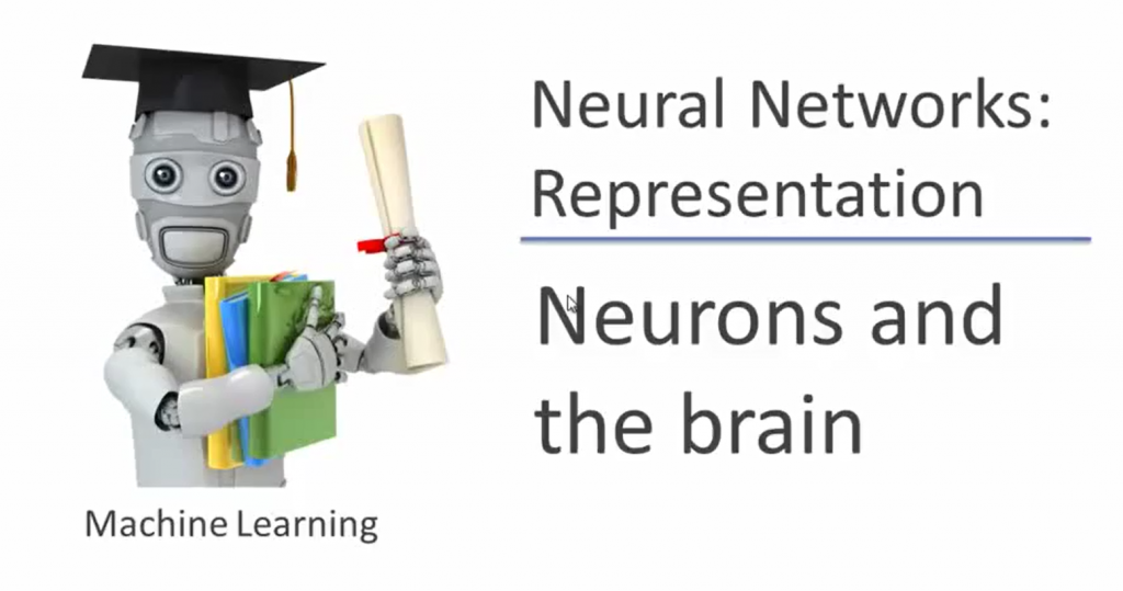
Well, I signed up for Andrew Ng’s Machine Learning Course at Stanford. It began a few weeks ago, and is a next generation to lectures by Ng circulating on YouTube. I’m going to basically audit the course, since I started a little late, but I plan to take several of the exams and work up a few of the projects. This course provides a broad introduction to machine learning, datamining, and statistical pattern recognition. Topics include: (i) Supervised learning (parametric/non-parametric algorithms, support vector machines, kernels, neural networks). (ii) Unsupervised learning (clustering, dimensionality reduction, recommender systems, deep learning). (iii) Best practices in machine learning (bias/variance theory; innovation process in machine learning and AI). The course will also draw from numerous case studies and applications, so that you’ll also learn how to apply learning algorithms to building smart robots (perception, control), text understanding (web search, anti-spam), computer vision, medical informatics, audio, database mining, and other areas. I like the change in format. The YouTube videos circulating on the web are lengthly, and involve Ng doing derivations on white boards. This is a more informal, expository format. Here is a link to a great short introduction to neural networks. Click on the link above this picture, since the picture itself does not trigger a YouTube. Ng’s introduction on this topic is fairly short, so here is the follow-on lecture, which starts the task of representing or modeling neural networks. I really like the way Ng approaches this is grounded in biology. I believe there is still time to sign up. Comment on Neural Networks and Machine Learning I can’t do much better than point to Professor Ng’s definition of machine learning – Machine learning is the science of getting computers to act without being explicitly programmed. In the past decade, machine learning has given us self-driving cars, practical speech recognition, effective web search, and a vastly improved understanding of the human genome. Machine learning is so pervasive today that you probably use it dozens of times a day without knowing it. Many researchers also think it is the best way to make progress towards human-level AI. In this class, you will learn about the most effective machine learning techniques, and gain practice implementing them and getting them to work for yourself. More importantly, you’ll learn about not only the theoretical underpinnings of learning, but also gain the practical know-how needed to quickly and powerfully apply these techniques to new problems. Finally, you’ll learn about some of Silicon Valley’s best practices in innovation as it pertains to machine learning and AI. And now maybe this is the future – the robot rock band.

accuracy of forecasts, artificial intelligence (AI), Bayesian methods, Big Data, bootstrapping, data science, energy forecasting, ensemble forecasts, predictive analytics

Global Energy Forecasting Competitions

June 18, 2014 Clive Jones

The 2012 Global Energy Forecasting Competition was organized by an IEEE Working Group to connect academic research and industry practice, promote analytics in engineering education, and prepare for forecasting challenges in the smart grid world. Participation was enhanced by alliance with Kaggle for the load forecasting track. There also was a second track for wind power forecasting.

Hundreds of people and many teams participated.

This year’s April/June issue of the International Journal of Forecasting (IJF) features research from the winners.

Before discussing the 2012 results, note that there’s going to be another competition – the Global Energy Forecasting Competition 2014 – scheduled for launch August 15 of this year. Professor Tao Hong, a key organizer, describes the expansion of scope,

GEFCom2014 (www.gefcom.org) will feature three major upgrades: 1) probabilistic forecasts in the form of predicted quantiles; 2) four tracks on demand, price, wind and solar; 3) rolling forecasts with incremental data update on weekly basis.

Results of the 2012 Competition

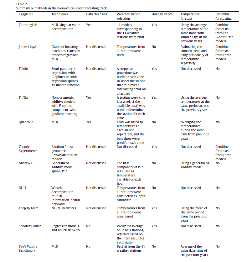
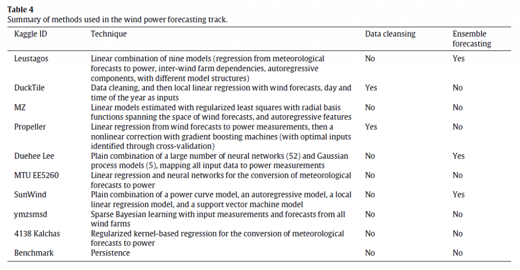
The IJF has an open source article on the competition. This features a couple of interesting tables about the methods in the load and wind power tracks (click to enlarge).

The error metric is WRMSE, standing for weighted root mean square error. One week ahead system (as opposed to zone) forecasts received the greatest weight. The top teams with respect to WRMSE were Quadrivio, CountingLab, James Lloyd, and Tololo (Électricité de France).

The top wind power forecasting teams were Leustagos, DuckTile, and MZ based on overall performance.

Innovations in Electric Power Load Forecasting

The IJF overview article pitches the hierarchical load forecasting problem as follows:

…participants were required to backcast and forecast hourly loads (in kW) for a US utility with 20 zones at both the zonal (20 series) and system (sum of the 20 zonal level series) levels, with a total of 21 series. We provided the participants with 4.5 years of hourly load and temperature history data, with eight non-consecutive weeks of load data removed. The backcasting task is to predict the loads of these eight weeks in the history, given actual temperatures, where the participants are permitted to use the entire history to backcast the loads. The forecasting task is to predict the loads for the week immediately after the 4.5 years of history without the actual temperatures or temperature forecasts being given. This is designed to mimic a short term load forecasting job, where the forecaster first builds a model using historical data, then develops the forecasts for the next few days.

One of the top entries is by a team from Électricité de France (EDF) and is written up under the title GEFCom2012: Electric load forecasting and backcasting with semi-parametric models.

This is behind the International Journal of Forecasting paywall at present, but some of the primary techniques can be studied in a slide set by Yannig Goulde.

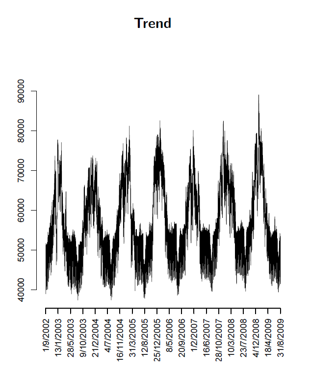
This is an interesting deck because it maps key steps in using semi-parametric models and illustrates real world system power load or demand data, as in this exhibit of annual variation showing the trend over several years.

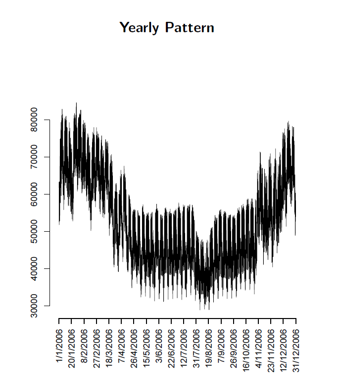
Or this exhibit showing annual variation.

What intrigues me about the EDF approach in the competition and, apparently, more generally in their actual load forecasting, is the use of splines and knots. I’ve seen this basic approach applied in other time series contexts, for example, to facilitate bagging estimates.

So these competitions seem to provide solid results which can be applied in a real-world setting.

Top image from Triple-Curve

Bayesian methods, Medical data analytics, predictive analytics

Bayesian Reasoning and Intuition

June 13, 2014 Clive Jones

In thinking about Bayesian methods, I wanted to focus on whether and how Bayesian probabilities are or can be made “intuitive.”

Or are they just numbers plugged into a formula which sometimes is hard to remember?

A classic example of Bayesian reasoning concerns breast cancer and mammograms.

1% of the women at age forty who participate in routine screening have breast cancer

80% of women with breast cancer will get positive mammograms.

9.6% of women with no breast cancer will also get positive mammograms

Question – A women in this age group has a positive mammogram in a routine screening. What is the probability she has cancer?

There is a tendency for intuition to anchor on the high percentage of women with breast cancer with positive mammograms – 80 percent. In fact, this type of scenario elicits significant over-estimates of cancer probabilities among mammographers!

Bayes Theorem, however, shows that the probability of women with a positive mammogram having cancer is an order of magnitude less than the percent of women with breast cancer and positive mammograms.

By the Formula

Recall Bayes Theorem –

Let A stand for the event a women has breast cancer, and B denote the event that a women tests positive on the mammogram.

We need the conditional probability of a positive mammogram, given that a woman has breast cancer, or P(B|A). In addition, we need the prior probability that a woman has breast cancer P(A), as well as the probability of a positive mammogram P(B).

So we know P(B|A)=0.8, and P(B|~A)=0.096, where the tilde ~ indicates “not”.

For P(B) we can make the following expansion, based on first principles –

P(B)=P(B|A)P(A)+P(B|~A)P(B)= P(B|A)P(A)+P(B|~A)(1-P(A))=0.10304

Either a woman has cancer or does not have cancer. The probability of a woman having cancer is P(A), so the probability of not having cancer is 1-P(A). These are mutually exclusive events, that is, and the probabilities sum to 1.

Putting the numbers together, we calculate the probability of a forty-year-old women with a positive mammogram having cancer is 0.0776.

So this woman has about an 8 percent chance of cancer, even though her mammogram is positive.

Survey after survey of physicians shows that this type of result in not very intuitive. Many doctors answer incorrectly, assigning a much higher probability to the woman having cancer.

Building Intuition

This example is the subject of a 2003 essay by Eliezer Yudkowsky – An Intuitive Explanation of Bayes’ Theorem.

As An Intuitive (and Short) Explanation of Bayes’ Theorem notes, Yudkowsky’s intuitive explanation is around 15,000 words in length.

For a shorter explanation that helps build intuition, the following table is useful, showing the crosstabs of women in this age bracket who (a) have or do not have cancer, and (b) who test positive or negative.

The numbers follow from our original data. The percentage of women with cancer who test positive is given as 80 percent, so the percent with cancer who test negative must be 20 percent, and so forth.

Now let’s embed the percentages of true and false positives and negatives into the table, as follows:

So 1 percent of forty year old women (who have routine screening) have cancer. If we multiply this 1 percent by the percent of women who have cancer and test positive, we get .008 or the chances of a true positive. Then, the chance of getting any type of positive result is .008+.99*.096=.008+.0954=0.10304.

The ratio then of the chances of a true positive to the chance of any type of positive result is 0.07763 – exactly the result following from Bayes Theorem!

This may be an easier two-step procedure than trying to develop conditional probabilities directly, and plug them into a formula.

Allen Downey lists other problems of this type, with YouTube talks on Bayesian stuff that are good for beginners.

Closing Comments

I have a couple more observations.

First, this analysis is consistent with a frequency interpretation of probability.

In fact, the 1 percent figure for women who are forty getting cancer could be calculated from cause of death data and Census data. Similarly with the other numbers in the scenario.

So that’s interesting.

Bayes theorem is, in some phrasing, true by definition (of conditional probability). It can just be tool for reorganizing data about observed frequencies.

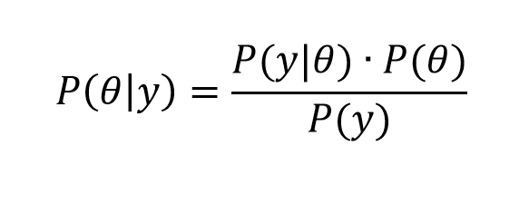
The magic comes when we transition from events to variables y and parameters θ in a version like,

What is this parameter θ? It certainly does not exist in “event” space in the same way as does the event of “having cancer and being a forty year old woman.” In the batting averages example, θ is a vector of parameter values of a Beta distribution – parameters which encapsulate our view of the likely variation of a batting average, given information from the previous playing season. So I guess this is where we go into “belief space”and subjective probabilities.

In my view, the issue is always whether these techniques are predictive.

Top picture courtesy of Siemens

accuracy of forecasts, Bayesian methods, bias in forecasts, regression diagnostics, ridge regression, the LASSO

Some Ways in Which Bayesian Methods Differ From the “Frequentist” Approach

June 12, 2014 Clive Jones

I’ve been doing a deep dive into Bayesian materials, the past few days. I’ve tried this before, but I seem to be making more headway this time.

One question is whether Bayesian methods and statistics informed by the more familiar frequency interpretation of probability can give different answers.

I found this question on CrossValidated, too – Examples of Bayesian and frequentist approach giving different answers.

Among other things, responders cite YouTube videos of John Kruschke – the author of Doing Bayesian Data Analysis A Tutorial With R and BUGS

Here is Kruschke’s “Bayesian Estimation Supercedes the t Test,” which, frankly, I recommend you click on after reading the subsequent comments here.

I guess my concern is not just whether Bayesian and the more familiar frequentist methods give different answers, but, really, whether they give different predictions that can be checked.

I get the sense that Kruschke focuses on the logic and coherence of Bayesian methods in a context where standard statistics may fall short.

But I have found a context where there are clear differences in predictive outcomes between frequentist and Bayesian methods.

This concerns Bayesian versus what you might call classical regression.

In lecture notes for a course on Machine Learning given at Ohio State in 2012, Brian Kulis demonstrates something I had heard mention of two or three years ago, and another result which surprises me big-time.

Let me just state this result directly, then go into some of the mathematical details briefly.

Suppose you have a standard ordinary least squares (OLS) linear regression, which might look like,

where we can assume the data for y and x are mean centered. Then, as is well, known, assuming the error process ε is N(0,σ) and a few other things, the BLUE (best linear unbiased estimate) of the regression parameters w is –

Now Bayesian methods take advantage of Bayes Theorem, which has a likelihood function and a prior probability on the right hand side of the equation, and the resulting posterior distribution on the left hand side of the equation.

What priors do we use for linear regression in a Bayesian approach?

Well, apparently, there are two options.

First, suppose we adopt priors for the predictors x, and suppose the prior is a normal distribution – that is the predictors are assumed to be normally distributed variables with various means and standard deviations.

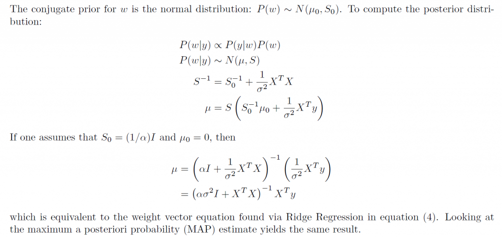
In this case, amazingly, the posterior distribution for a Bayesian setup basically gives the equation for ridge regression.

On the other hand, assuming a prior which is a Laplace distribution gives a posterior distribution which is equivalent to the lasso.

This is quite stunning, really.

Obviously, then, predictions from an OLS regression, in general, will be different from predictions from a ridge regression estimated on the same data, depending on the value of the tuning parameter λ (See the post here on this).

Similarly with a lasso regression – different forecasts are highly likely.

Now it’s interesting to question which might be more accurate – the standard OLS or the Bayesian formulations. The answer, of course, is that there is a tradeoff between bias and variability effected here. In some situations, ridge regression or the lasso will produce superior forecasts, measured, for example, by root mean square error (RMSE).

This is all pretty wonkish, I realize. But it conclusively shows that there can be significant differences in regression forecasts between the Bayesian and frequentist approaches.

What interests me more, though, is Bayesian methods for forecast combination. I am still working on examples of these procedures. But this is an important area, and there are a number of studies which show gains in forecast accuracy, measured by conventional metrics, for Bayesian model combinations.

accuracy of forecasts, Bayesian methods, conjugate prior

Predicting Season Batting Averages, Bernoulli Processes – Bayesian vs Frequentist

June 10, 2014 Clive Jones

Recently, Nate Silver boosted Bayesian methods in his popular book The Signal and the Noise – Why So Many Predictions Fail – But Some Don’t. I’m guessing the core application for Silver is estimating batting averages. Silver first became famous with PECOTA, a system for forecasting the performance of Major League baseball players.

Let’s assume a player’s probability p of getting a hit is constant over a season, but that it varies from year to year. He has up years, and down years. And let’s compare frequentist (gnarly word) and Bayesian approaches at the beginning of the season.

The frequentist approach is based on maximum likelihood estimation with the binomial formula

Here the n and the k in parentheses at the beginning of the expression stand for the combination of n things taken k at a time. That is, the number of possible ways of interposing k successes (hits) in n trials (times at bat) is the combination of n things taken k at a time (formula here).

If p is the player’s probability of hitting at bat, then the entire expression is the probability the player will have k hits in n times at bat.

The Frequentist Approach

There are a couple of ways to explain the frequentist perspective.

One is that this binomial expression is approximated to a higher and higher degree of accuracy by a normal distribution. This means that – with large enough n – the ratio of hits to total times at bat is the best estimate of the probability of a player hitting at bat – or k/n.

This solution to the problem also can be shown to follow from maximizing the likelihood of the above expression for any n and k. The large sample or asymptotic and maximum likelihood solutions are numerically identical.

The problem comes with applying this estimate early on in the season. So if the player has a couple of rough times at bat initially, the frequentist estimate of his batting average for the season at that point is zero.

The Bayesian Approach

The Bayesian approach is based on the posterior probability distribution for the player’s batting average. From Bayes Theorem, this is a product of the likelihood and a prior for the batting average.

Now generally, especially if we are baseball mavens, we have an idea of player X’s batting average. Say we believe it will be .34 – he’s going to have a great season, and did last year.

In this case, we can build that belief or information into a prior that is a beta distribution with two parameters α and β that generate a mean of α/(α+β).

In combination with the binomial likelihood function, this beta distribution prior combines algebraically into a closed form expression for another beta function with parameters which are adjusted by the values of k and n-k (the number of strike-outs). Note that walks (also being hit by the ball) do not count as times at bat.

This beta function posterior distribution then can be moved back to the other side of the Bayes equation when there is new information – another hit or strikeout.

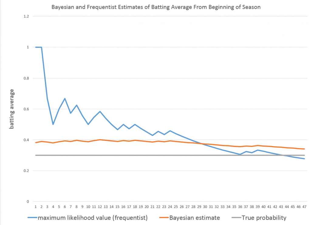
Taking the average of the beta posterior as the best estimate of p, then, we get successive approximations, such as shown in the following graph.

So the player starts out really banging ‘em, and the frequentist estimate of his batting average for that season starts at 100 percent. The Bayesian estimate on the other hand is conditioned by a belief that his batting average should be somewhere around 0.34. In fact, as the grey line indicates, his actual probability p for that year is 0.3. Both the frequentist and Bayesian estimates converge towards this value with enough times at bat.

I used α=33 and β=55 for the initial values of the Beta distribution.

See this for a great discussion of the intuition behind the Beta distribution.

This, then, is a worked example showing how Bayesian methods can include prior information, and have small sample properties which can outperform a frequentist approach.

Of course, in setting up this example in a spreadsheet, it is possible to go on and generate a large number of examples to explore just how often the Bayesian estimate beats the frequentist estimate in the early part of a Bernoulli process.

Which goes to show that what you might call the classical statistical approach – emphasizing large sample properties, covering all cases, still has legs.

Business Forecasting