Friends and acquaintances know that I believe I have discovered amazing, deep, and apparently simple predictability in aspects of the daily, weekly, monthly movement of stock prices.
People say – “don’t blog about it, keep it to yourself, and use it to make a million dollars.” That does sound attractive, but I guess I am a data scientist, rather than stock trader. Not only that, but the pattern looks to be self-fulfilling. Generally, the result of traders learning about this pattern should be to reinforce, rather than erase, it. There seems to be no other explanation consistent with its long historical vintage, nor the broadness of its presence. And that is big news to those of us who like to linger in the forecasting zoo.
I am going to share my discovery with you, at least in part, in this blog post.
But first, let me state some ground rules and describe the general tenor of my analysis. I am using OLS regression in spreadsheets at first, to explore the data. I am only interested, really, in models which have significant out-of-sample prediction capabilities. This means I estimate the regression model over a set of historical data and then use that model to predict – in this case the high and low of the SPY exchange traded fund. The predictions (or “retrodictions” or “backcasts”) are for observations on the high and low stock prices for various periods not included in the data used to estimate the model.
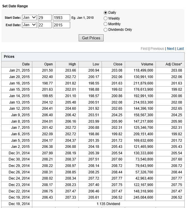
Now let’s look at the sort of data I use. The following table is from Yahoo Finance for the SPY. The site allows you to download this data into a spreadsheet, although you have to invert the order of the dating with a sort on the date. Note that all data is for trading days, and when I speak of N-day periods in the following, I mean periods of N trading days.
OK, now let me state my major result.
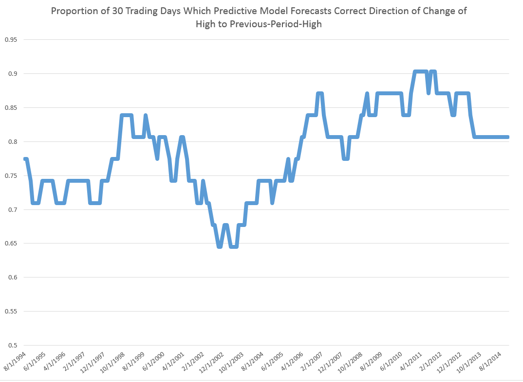
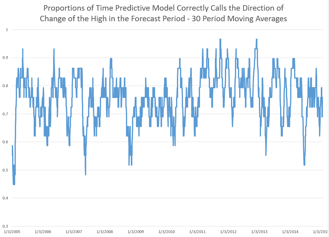
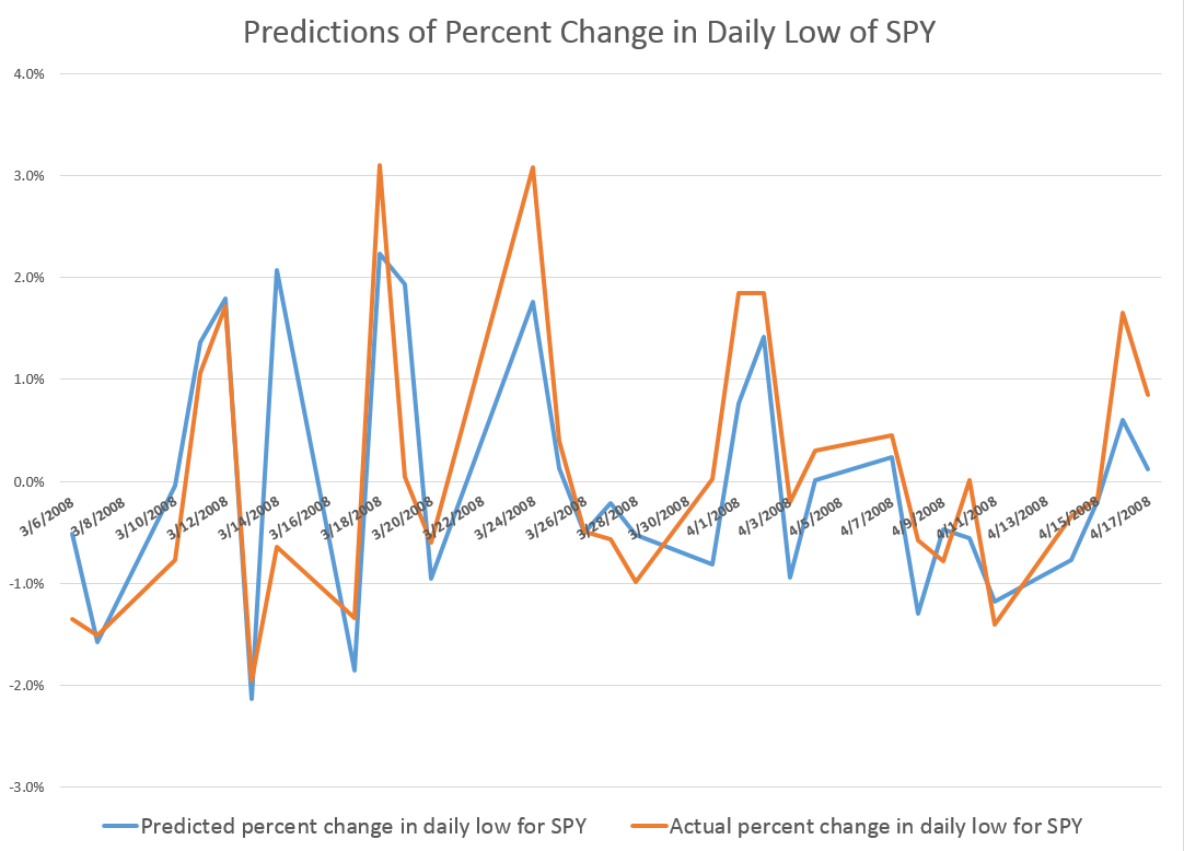
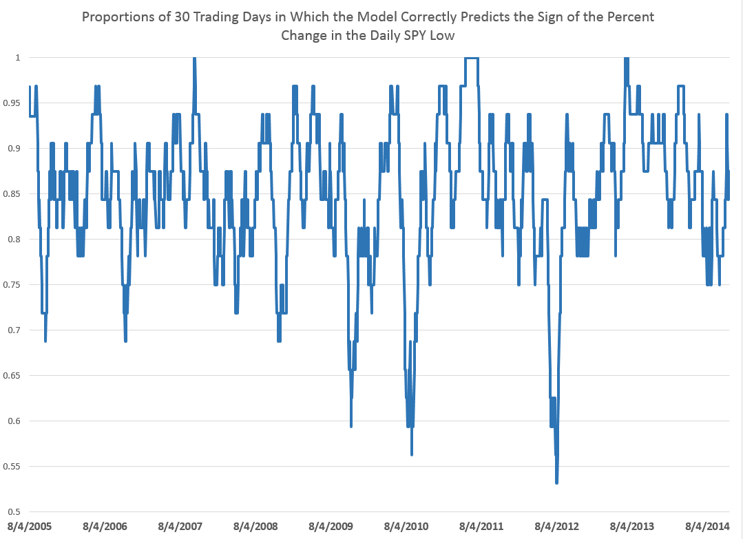
For every period from daily periods to 60 day periods I have investigated, the high and low prices are “relatively” predictable and the direction of change from period to period is predictable, in backcasting analysis, about 70-80 percent of the time, on average.
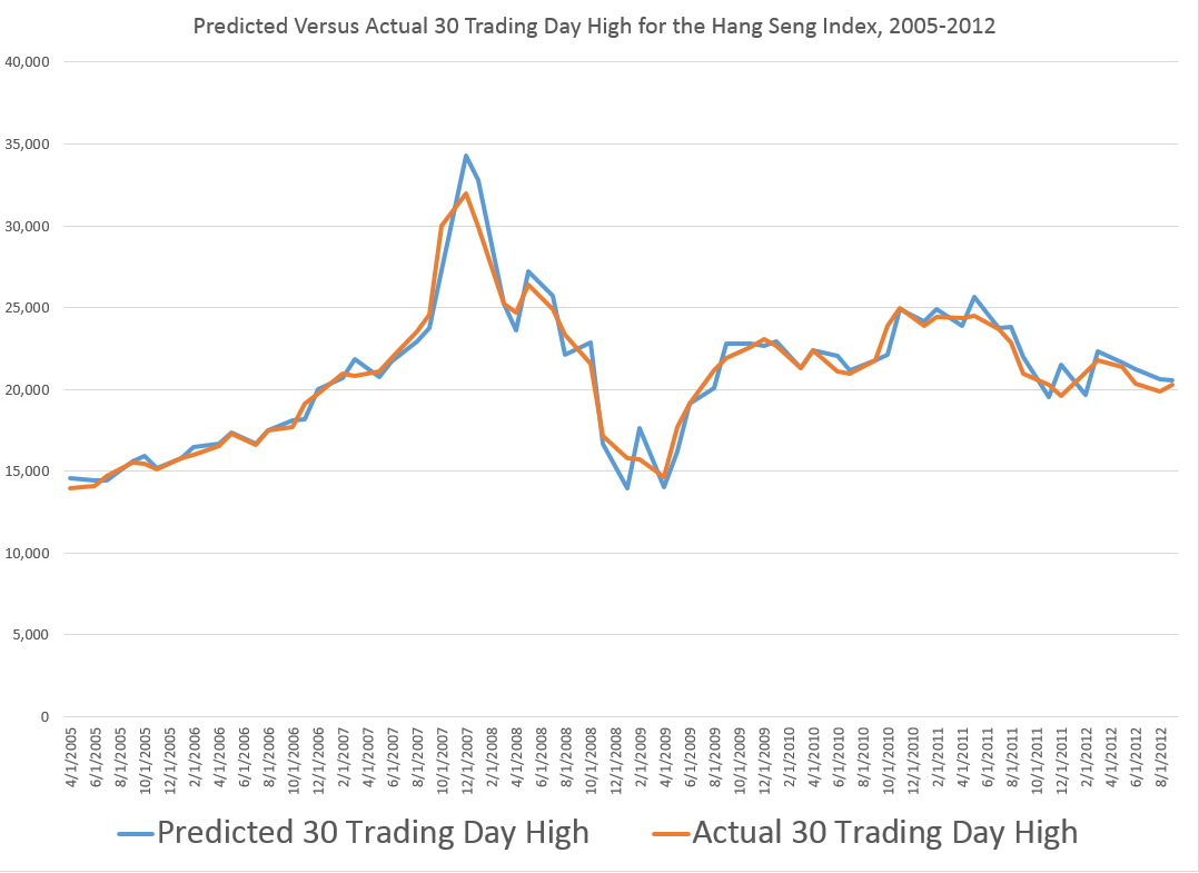
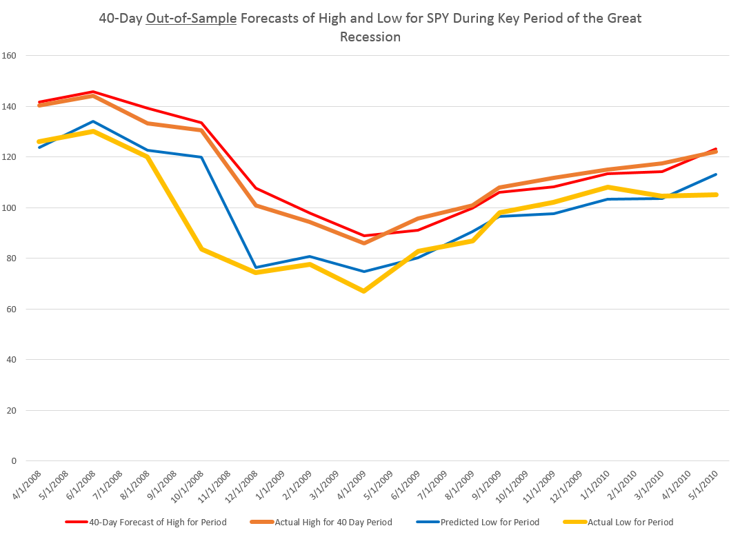
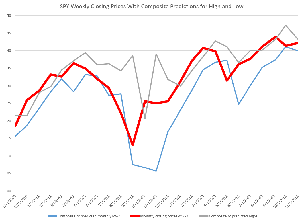
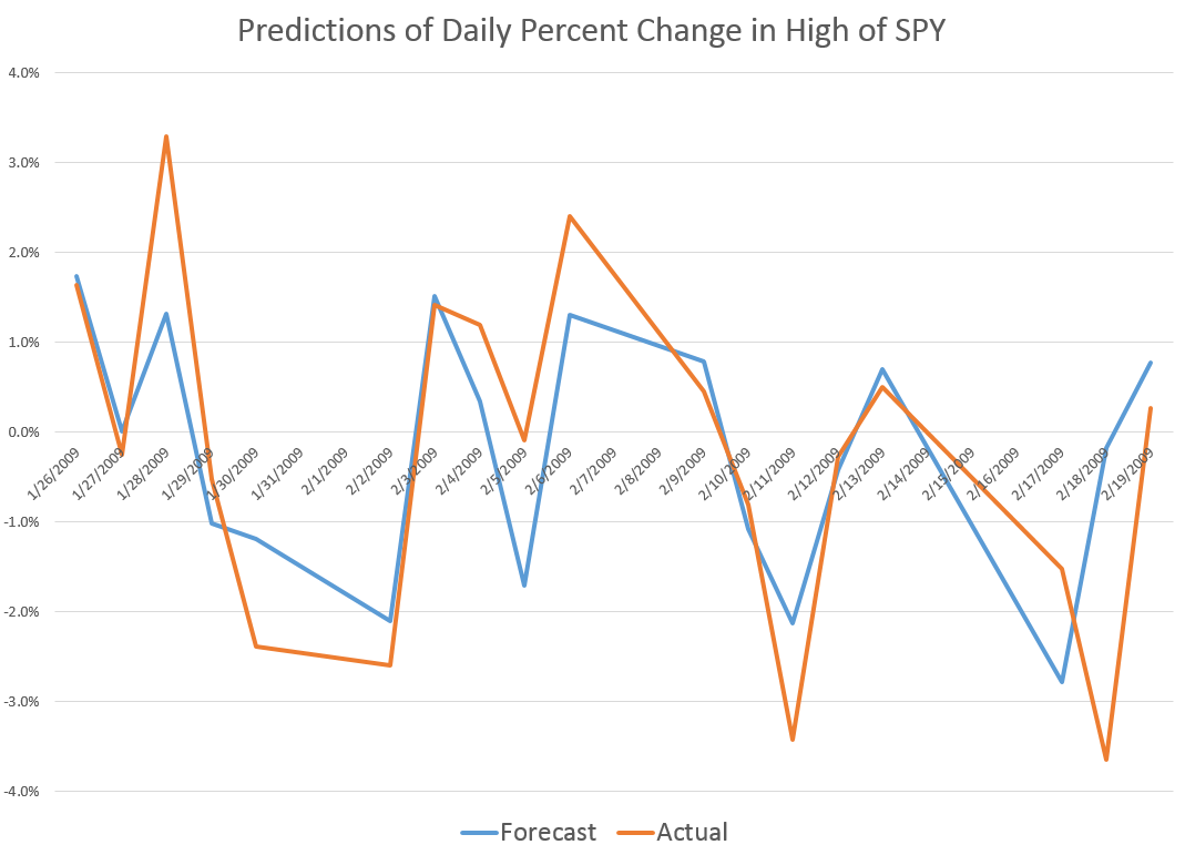
To give an example of a backcasting analysis, consider this chart from the period of free-fall in markets during 2008-2009, the Great Recession (click to enlarge).
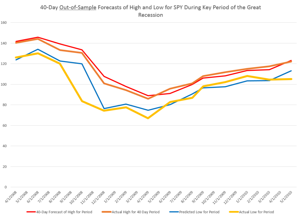
Now note that the indicated lines for the forecasts are not, strictly-speaking, 40-day-ahead forecasts. The forecasts are for the level of the high and low prices of the SPY which will be attained in each period of 40 trading days.
But the point is these rather time-indeterminate forecasts, when graphed alongside the actual highs and lows for the 40 trading day periods in question, are relatively predictive.
More to the point, the forecasts suffice to signal a key turning point in the SPY. Of course, it is simple to relate the high and low of the SPY for a period to relevant measures of the average or closing stock prices.
So seasoned forecasters and students of the markets and economics should know by this example that we are in terra incognita. Forecasting turning points out-of-sample is literally the toughest thing to do in forecasting, and certain with respect to the US stock market.
Many times technical analysts claim to predict turning points, but their results may seem more artistic, involving subtle interpretations of peaks and shoulders, as well as levels of support.
Now I don’t want to dismiss technical analysis, since, indeed, I believe my findings may prove out certain types of typical results in technical analysis. Or at least I can see a way to establish that claim, if things work out empirically.
Forecast of SPY High And Low for the Next Period of 40 Trading Days
What about the coming period of 40 trading days, starting from this morning’s (January 22, 2015) opening price for the SPY – $203.99?
Well, subject to qualifications I will state further on here, my estimates suggest the high for the period will be in the range of $215 and the period low will be around $194. Cents attached to these forecasts would be, of course, largely spurious precision.
In my opinion, these predictions are solid enough to suggest that no stock market crash is in the cards over the next 40 trading days, nor will there be a huge correction. Things look to trade within a range not too distant from the current situation, with some likelihood of higher highs.
It sounds a little like weather forecasting.
The Basic Model
Here is the actual regression output for predicting the 40 trading day high of the SPY.
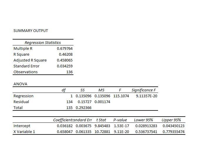
This is a simpler than many of the models I have developed, since it only relies on one explanatory variable designated X Variable 1 in the Excel regression output. This explanatory variable is the ratio of the current opening price to the previous high for the 40 day trading period, all minus 1.
Let’s call this -1+ O/PH. Instances of -1+ O/PH are generated for data bunched by 40 trading day periods, and put into the regression against the growth in consecutive highs for these 40 day periods.
So what happens is this, apparently.
Everything depends on the opening price. If the high for the previous period equals the opening price, the predicted high for the next 40 day period will be the same as the high for the previous 40 day period.
If the previous high is less than the opening price, the prediction is that the next period high will be higher. Otherwise, the prediction is that the next period high will be lower.
This then looks like a trading rule which even the numerically challenged could follow.
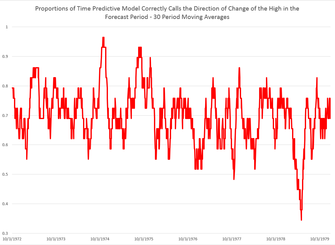
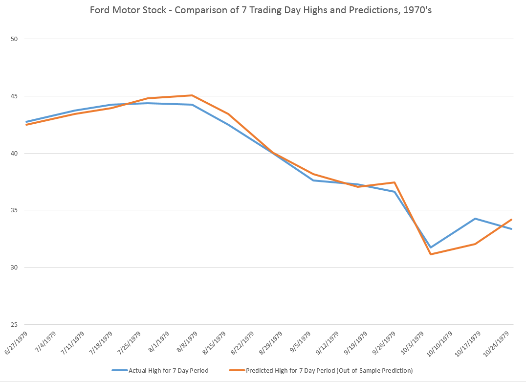
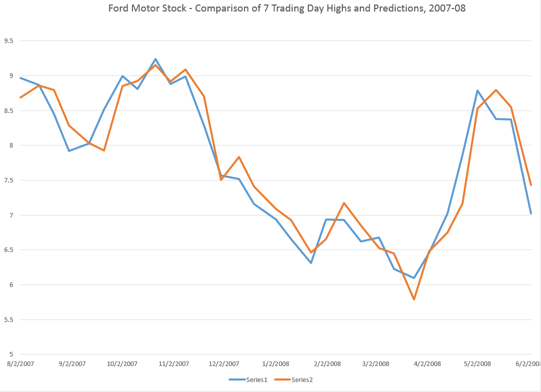
And this sort of relationship is not something that has just emerged with quants and high frequency trading. On the contrary, it is possible to find the same type of rule operating with, say, Exxon’s stock (XOM) in the 1970’s and 1980’s.
But, before jumping to test this out completely, understand that the above regression is, in terms of most of my analysis, partial, missing at least one other important explanatory variable.
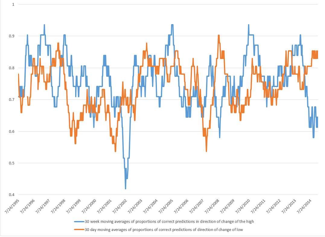
Previous posts, which employ similar forecasting models for daily, weekly, and monthly trading periods, show that these models can predict the direction of change of the period highs with about 70 to 80 percent accuracy (See, for example, here).
Provisos and Qualifications
In deploying OLS regression analysis, in Excel spreadsheets no less, I am aware there are many refinements which, logically, might be developed and which may improve forecast accuracy.
One thing I want to stress is that residuals of the OLS regressions on the growth in the period highs generally are not normally distributed. The distribution tends to be very peaked, reminiscent of discussions earlier in this blog of the Laplace distribution for Microsoft stock prices.
There also is first order serial correlation in many of these regressions. And, my software indicates that there could be autocorrelations extending deep into the historical record.
Finally, the regression coefficients may vary over the historical record.
Bottom LIne
I like Robb Hyndman’s often drawn distinction between modeling and reality. Somewhere Hyndman suggests that no model is right.
But this class of models has an extremely logical motivation, and is, as I say, relatively predictive – predictive enough to be useful in a number of contexts.
Momentum traders for years apparently have looked at the opening price and compared it with the highs (and lows) for previous periods – extending 60 days or more into history if not more – and decided whether to trade. If the opening price is greater than the past high, the next high is anticipated to be even higher. On this basis, stock may be purchased. That action tends to reinforce the relationship. So, in some sense, this is a self-fulfilling relationship.
To recapitulate – I can show you iron-clad, incontrovertible evidence that some fairly simple models built on daily trading data produce workable forecasts of the high and low for stock indexes and stocks. These forecasts are available for a variety of time periods, and, apparently, in backcasts can indicate turning points in the market.
As I say, feel free to request further documentation. I am preparing a write-up for a journal, and I think I can find a way to send out versions of this.
You can contact me confidentially via the Comments box below. Leave your email or phone number. Title the Comment “Request for High/Low Model Information” and the webmeister will forward it to me without having your request listed in the side panel of the blog.