Tag Archives: bagging

Revisiting the Predictability of the S&P 500

Almost exactly a year ago, I posted on an algorithm and associated trading model for the S&P 500, the stock index which supports the SPY exchange traded fund.

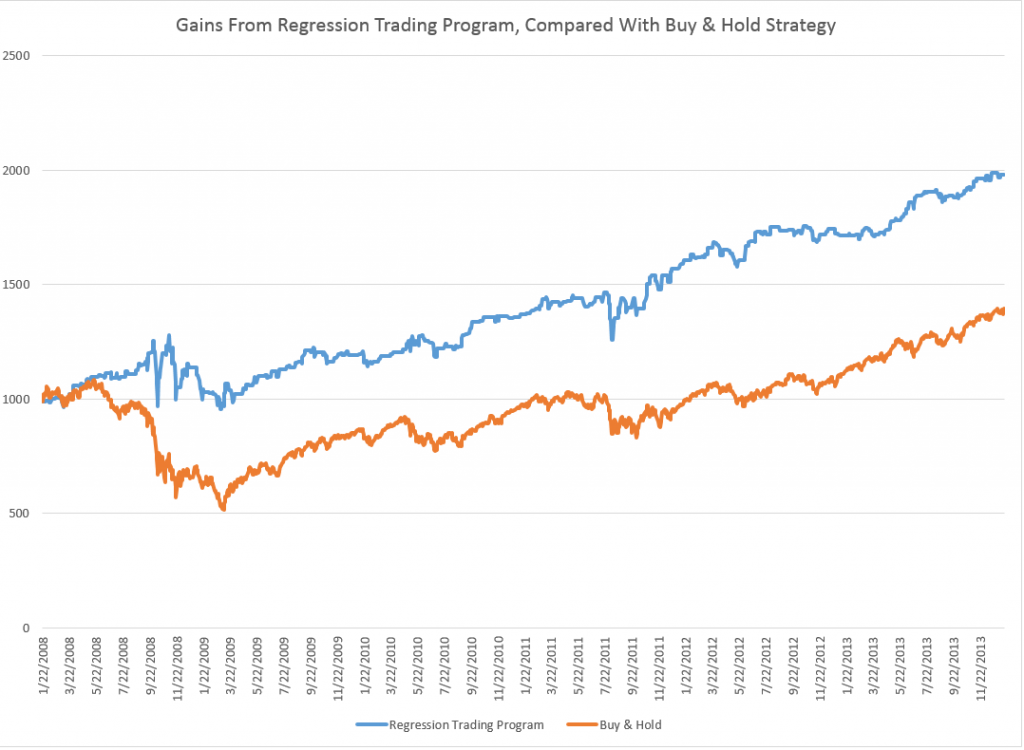
I wrote up an autoregressive (AR) model, using daily returns for the S&P 500 from 1993 to early 2008. This AR model outperforms a buy-and-hold strategy for the period 2008-2013, as the following chart shows.

SPYTradingProgramcompBH

The trading algorithm involves “buying the S&P 500” when the closing price indicates a positive return for the following trading day. Then, I “close out the investment” the next trading day at that day’s closing price. Otherwise, I stay in cash.

It’s important to be your own worst critic, and, along those lines, I’ve had the following thoughts.

First, the above graph disregards trading costs. Your broker would have to be pretty forgiving to execute 2000-3000 trades for less than the $500 you make over the buy-and-hold strategy. SO, I should deduct something for the trades in calculating the cumulative value.

The other criticism concerns high frequency trading. The daily returns are calculated against closing values, but, of course, to use this trading system you have to trade prior to closing. However, even a few seconds can make a crucial difference in the price of the S&P 500 or SPY – and even smaller intervals.

An Up-Dated AR Model

Taking some of these criticisms into account, I re-estimate an autoregressive model on more recent data –again calculating returns against closing prices on successive trading days.

This time I start with an initial investment of $100,000, and deduct $5 per trade off the totals as they cumulate.

I also utilize only seven (7) lags for the daily returns. This compares with the 30 lag model from the post a year ago, and I estimate the current model with OLS, rather than maximum likelihood.

The model is

Rt = 0.0007-0.0651Rt-1+0.0486Rt-2-0.0999Rt-3-0.0128Rt-4-0.1256Rt-5 +0.0063Rt-6-0.0140Rt-7

where Rt is the daily return for trading day t. This model originates on data from June 11, 2011. The coefficients of the equation result from bagging OLS regressions – developing coefficient estimates for 100,000 similar size samples drawn with replacement from this dataset of 809 observations. These 100,000 coefficient estimates are averaged to arrive at the numbers shown above.

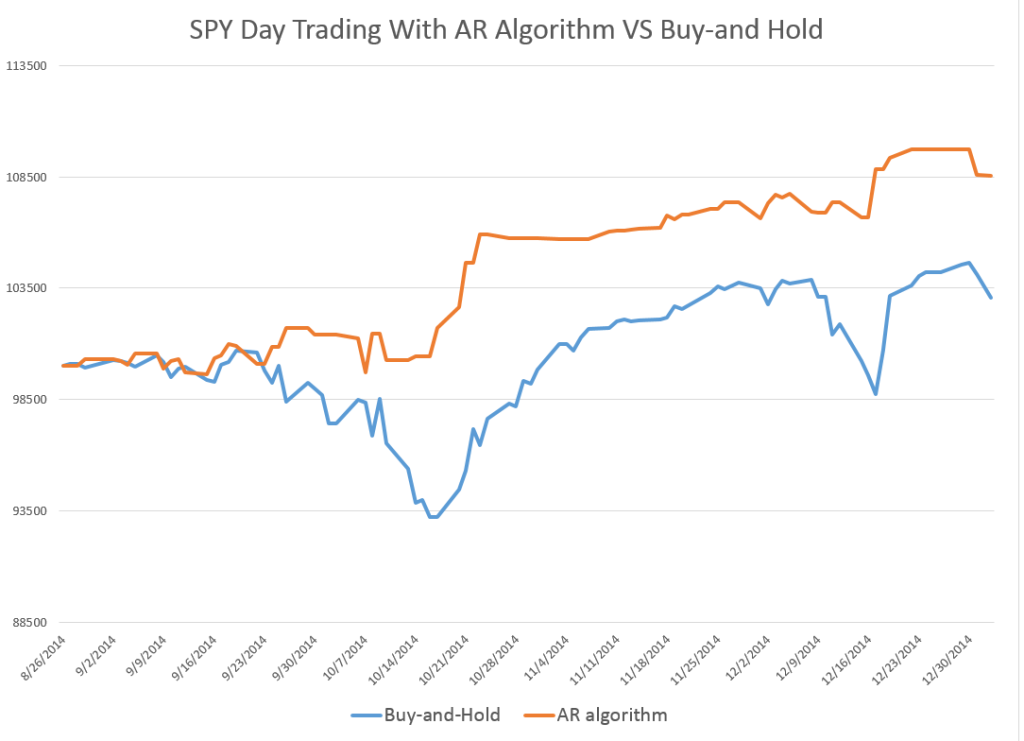
Here is the result of applying my revised model to recent stock market activity. The results are out-of-sample. In other words, I use the predictive equation which is calculated over data prior to the start of the investment comparison. I also filter the positive predictions for the next day closing price, only acting when they are a certain size or larger.

NewARmodel

There is a 2-3 percent return on a hundred thousand dollar investment in one month, and a projected annual return on the order of 20-30 percent.

The current model also correctly predicts the sign of the daily return 58 percent of the time, compared with a much lower figure for the model from a year ago.

This looks like the best thing since sliced bread.

But wait – what about high frequency trading?

I’m exploring the implementation of this model – and maybe should never make it public.

But let me clue you in on what I suspect, and some evidence I have.

So, first, it is interesting the gains from trading on closing day prices more than evaporate by the opening of the New York Stock Exchange, following the generation of a “buy” signal according to this algorithm.

In other words, if you adjust the trading model to buy at the open of the following trading day, when the closing price indicates a positive return for the following day – you do not beat a buy-and-hold strategy. Something happens between the closing and the opening of the NYSE market for the SPY.

Someone else knows about this model?

I’m exploring the “final second’ volatility of the market, focusing on trading days when the closing prices look like they might come in to indicate a positive return the following day. This is complicated, and it puts me into issues of predictability in high frequency data.

I also am looking at the SPY numbers specifically to bring this discussion closer to trading reality.

Bottom line – It’s hard to make money in the market on trading algorithms if you are a day-trader – although probably easier with a super-computer at your command and when you sit within microseconds of executing an order on the NY Stock Exchange.

But these researches serve to indicate one thing fairly clearly. And that is that there definitely are aspects of stock prices which are predictable. Acting on the predictions is the hard part.

And Postscript: Readers may have noticed a lesser frequency of posting on Business Forecast blog in the past week or so. I am spending time running estimations and refreshing and extending my understanding of some newer techniques. Keep checking in – there is rapid development in “real world forecasting” – exciting and whiz bang stuff. I need to actually compute the algorithms to gain a good understanding – and that is proving time-consuming. There is cool stuff in the data warehouse though.
Wrap on Exponential Smoothing

Here are some notes on essential features of exponential smoothing.

  1. Name. Exponential smoothing (ES) algorithms create exponentially weighted sums of past values to produce the next (and subsequent period) forecasts. So, in simple exponential smoothing, the recursion formula is Lt=αXt+(1-α)Lt-1 where α is the smoothing constant constrained to be within the interval [0,1], Xt is the value of the time series to be forecast in period t, and Lt is the (unobserved) level of the series at period t. Substituting the similar expression for Lt-1 we get Lt=αXt+(1-α) (αXt-1+(1-α)Lt-2)= αXt+α(1-α)Xt-1+(1-α)2Lt-2, and so forth back to L1. This means that more recent values of the time series X are weighted more heavily than values at more distant times in the past. Incidentally, the initial level L1 is not strongly determined, but is established by one ad hoc means or another – often by keying off of the initial values of the X series in some manner or another. In state space formulations, the initial values of the level, trend, and seasonal effects can be included in the list of parameters to be established by maximum likelihood estimation.
  2. Types of Exponential Smoothing Models. ES pivots on a decomposition of time series into level, trend, and seasonal effects. Altogether, there are fifteen ES methods. Each model incorporates a level with the differences coming as to whether the trend and seasonal components or effects exist and whether they are additive or multiplicative; also whether they are damped. In addition to simple exponential smoothing, Holt or two parameter exponential smoothing is another commonly applied model. There are two recursion equations, one for the level Lt and another for the trend Tt, as in the additive formulation, Lt=αXt+(1-α)(Lt-1+Tt-1) and Tt=β(Lt– Lt-1)+(1-β)Tt-1 Here, there are now two smoothing parameters, α and β, each constrained to be in the closed interval [0,1]. Winters or three parameter exponential smoothing, which incorporates seasonal effects, is another popular ES model.
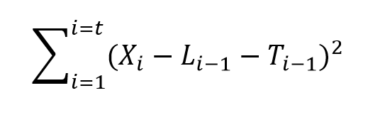
  3. Estimation of the Smoothing Parameters. The original method of estimating the smoothing parameters was to guess their values, following guidelines like “if the smoothing parameter is near 1, past values will be discounted further” and so forth. Thus, if the time series to be forecast was very erratic or variable, a value of the smoothing parameter which was closer to zero might be selected, to achieve a longer period average. The next step is to set up a sum of the squared differences of the within sample predictions and minimize these. Note that the predicted value of Xt+1 in the Holt or two parameter additive case is Lt+Tt, so this involves minimizing the expression Sqerroreq Currently, the most advanced method of estimating the value of the smoothing parameters is to express the model equations in state space form and utilize maximum likelihood estimation. It’s interesting, in this regard, that the error correction version of ES recursion equations are a bridge to this approach, since the error correction formulation is found at the very beginnings of the technique. Advantages of using the state space formulation and maximum likelihood estimation include (a) the ability to estimate confidence intervals for point forecasts, and (b) the capability of extending ES methods to nonlinear models.
  4. Comparison with Box-Jenkins or ARIMA models. ES began as a purely applied method developed for the US Navy, and for a long time was considered an ad hoc procedure. It produced forecasts, but no confidence intervals. In fact, statistical considerations did not enter into the estimation of the smoothing parameters at all, it seemed. That perspective has now changed, and the question is not whether ES has statistical foundations – state space models seem to have solved that. Instead, the tricky issue is to delineate the overlap and differences between ES and ARIMA models. For example, Gardner makes the statement that all linear exponential smoothing methods have equivalent ARIMA models. Hyndman points out that the state space formulation of ES models opens the way for expressing nonlinear time series – a step that goes beyond what is possible in ARIMA modeling.
  5. The Importance of Random Walks. The random walk is a forecasting benchmark. In an early paper, Muth showed that a simple exponential smoothing model provided optimal forecasts for a random walk. The optimal forecast for a simple random walk is the current period value. Things get more complicated when there is an error associated with the latent variable (the level). In that case, the smoothing parameter determines how much of the recent past is allowed to affect the forecast for the next period value.
  6. Random Walks With Drift. A random walk with drift, for which a two parameter ES model can be optimal, is an important form insofar as many business and economic time series appear to be random walks with drift. Thus, first differencing removes the trend, leaving ideally white noise. A huge amount of ink has been spilled in econometric investigations of “unit roots” – essentially exploring whether random walks and random walks with drift are pretty much the whole story when it comes to major economic and business time series.
  7. Advantages of ES. ES is relatively robust, compared with ARIMA models, which are sensitive to mis-specification. Another advantage of ES is that ES forecasts can be up and running with only a few historic observations. This comment applied to estimation of the level and possibly trend, but does not apply in the same degree to the seasonal effects, which usually require more data to establish. There are a number of references which establish the competitive advantage in terms of the accuracy of ES forecasts in a variety of contexts.
  8. Advanced Applications.The most advanced application of ES I have seen is the research paper by Hyndman et al relating to bagging exponential smoothing forecasts.

The bottom line is that anybody interested in and representing competency in business forecasting should spend some time studying the various types of exponential smoothing and the various means to arrive at estimates of their parameters.

For some reason, exponential smoothing reaches deep into actual process in data generation and consistently produces valuable insights into outcomes.

Bootstrapping

I’ve been reading about the bootstrap. I’m interested in bagging or bootstrap aggregation.

The primary task of a statistician is to summarize a sample based study and generalize the finding to the parent population in a scientific manner..

The purpose of a sample study is to gather information cheaply in a timely fashion. The idea behind bootstrap is to use the data of a sample study at hand as a “surrogate population”, for the purpose of approximating the sampling distribution of a statistic; i.e. to resample (with replacement) from the sample data at hand and create a large number of “phantom samples” known as bootstrap samples. The sample summary is then computed on each of the bootstrap samples (usually a few thousand). A histogram of the set of these computed values is referred to as the bootstrap distribution of the statistic.

These well-phrased quotes come from Bootstrap: A Statistical Method by Singh and Xie.

OK, so let’s do a simple example.

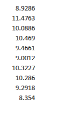
Suppose we generate ten random numbers, drawn independently from a Gaussian or normal distribution with a mean of 10 and standard deviation of 1.

vector

This sample has an average of 9.7684. We would like to somehow project a 95 percent confidence interval around this sample mean, to understand how close it is to the population average.

So we bootstrap this sample, drawing 10,000 samples of ten numbers with replacement.

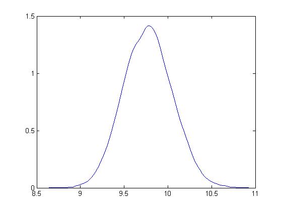
Here is the distribution of bootstrapped means of these samples.

bootstrapdist

The mean is 9.7713.

Based on the method of percentiles, the 95 percent confidence interval for the sample mean is between 9.32 and 10.23, which, as you note, correctly includes the true mean for the population of 10.

Bias-correction is another primary use of the bootstrap. For techies, there is a great paper from the old Bell Labs called A Real Example That Illustrates Properties of Bootstrap Bias Correction. Unfortunately, you have to pay a fee to the American Statistical Association to read it – I have not found a free copy on the Web.

In any case, all this is interesting and a little amazing, but what we really want to do is look at the bootstrap in developing forecasting models.

Bootstrapping Regressions

There are several methods for using bootstrapping in connection with regressions.

One is illustrated in a blog post from earlier this year. I treated the explanatory variables as variables which have a degree of randomness in them, and resampled the values of the dependent variable and explanatory variables 200 times, finding that doing so “brought up” the coefficient estimates, moving them closer to the underlying actuals used in constructing or simulating them.

This method works nicely with hetereoskedastic errors, as long as there is no autocorrelation.

Another method takes the explanatory variables as fixed, and resamples only the residuals of the regression.

Bootstrapping Time Series Models

The underlying assumptions for the standard bootstrap include independent and random draws.

This can be violated in time series when there are time dependencies.

Of course, it is necessary to transform a nonstationary time series to a stationary series to even consider bootstrapping.

But even with a time series that fluctuates around a constant mean, there can be autocorrelation.

So here is where the block bootstrap can come into play. Let me cite this study – conducted under the auspices of the Cowles Foundation (click on link) – which discusses the asymptotic properties of the block bootstrap and provides key references.

There are many variants, but the basic idea is to sample blocks of a time series, probably overlapping blocks. So if a time series yt  has n elements, y1,..,yn and the block length is m, there are n-m blocks, and it is necessary to use n/m of these blocks to construct another time series of length n. Issues arise when m is not a perfect divisor of n, and it is necessary to develop special rules for handling the final values of the simulated series in that case.

Block bootstrapping is used by Bergmeir, Hyndman, and Benıtez in bagging exponential smoothing forecasts.

How Good Are Bootstrapped Estimates?

Consistency in statistics or econometrics involves whether or not an estimate or measure converges to an unbiased value as sample size increases – or basically goes to infinity.

This is a huge question with bootstrapped statistics, and there are new findings all the time.

Interestingly, sometimes bootstrapped estimates can actually converge faster to the appropriate unbiased values than can be achieved simply by increasing sample size.

And some metrics really do not lend themselves to bootstrapping.

Also some samples are inappropriate for bootstrapping.  Gelman, for example, writes about the problem of “separation” in a sample

[In} ..an example of a poll from the 1964 U.S. presidential election campaign, … none of the black respondents in the sample supported the Republican candidate, Barry Goldwater… If zero black respondents in the sample supported Barry Goldwater, then zero black respondents in any bootstrap sample will support Goldwater as well. Indeed, bootstrapping can exacerbate separation by turning near-separation into complete separation for some samples. For example, consider a survey in which only one or two of the black respondents support the Republican candidate. The resulting logistic regression estimate will be noisy but it will be finite.

Here is a video doing a good job of covering the bases on boostrapping. I suggest sampling portions of it first. It’s quite good, but it may seem too much going into it.

Bagging Exponential Smoothing Forecasts

Bergmeir, Hyndman, and Benıtez (BHB) successfully combine two powerful techniques – exponential smoothing and bagging (bootstrap aggregation) – in ground-breaking research.

I predict the forecasting system described in Bagging Exponential Smoothing Methods using STL Decomposition and Box-Cox Transformation will see wide application in business and industry forecasting.

These researchers demonstrate their algorithms for combining exponential smoothing and bagging outperform all other forecasting approaches in the M3 forecasting competition database for monthly time series, and do better than many approaches for quarterly and annual data. Furthermore, the BHB approach can be implemented with extant routines in the programming language R.

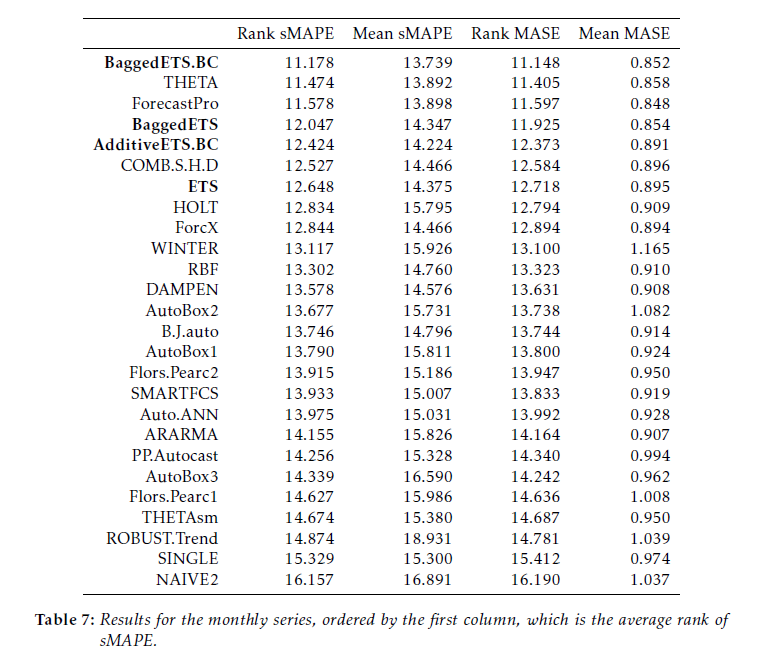
This table compares bagged exponential smoothing with other approaches on monthly data from the M3 competition.

BaggedES

Here BaggedETS.BC refers to a variant of the bagged exponential smoothing model which uses a Box Cox transformation of the data to reduce the variance of model disturbances, The error metrics are the symmetric mean absolute percentage error (sMAPE) and the mean absolute scaled error (MASE). These are calculated for applications of the various models to out-of-sample, holdout, or test sample data from each of 1428 monthly time series in the competition.

See the online text by Hyndman and Athanasopoulos for motivations and discussions of these error metrics.

The BHB Algorithm

In a nutshell, here is the BHB description of their algorithm.

After applying a Box-Cox transformation to the data, the series is decomposed into trend, seasonal and remainder components. The remainder component is then bootstrapped using the MBB, the trend and seasonal components are added back, and the Box-Cox transformation is inverted. In this way, we generate a random pool of similar bootstrapped time series. For each one of these bootstrapped time series, we choose a model among several exponential smoothing models, using the bias-corrected AIC. Then, point forecasts are calculated using all the different models, and the resulting forecasts are averaged.

The MBB is the moving block bootstrap. It involves random selection of blocks of the remainders or residuals, preserving the time sequence and, hence, autocorrelation structure in these residuals.

Several R routines supporting these algorithms have previously been developed by Hyndman et al. In particular, the ets routine developed by Hyndman and Khandakar fits 30 different exponential smoothing models to a time series, identifying the optimal model by an Akaike information criterion.

Some Thoughts

This research lays out an almost industrial-scale effort to extract more information for prediction purposes from time series, and at the same time to use an applied forecasting workhorse – exponential smoothing.

Exponential smoothing emerged as a forecasting technique in applied contexts in the 1950’s and 1960’s. The initial motivation was error correction from forecasts of arbitrary origin, instead of an underlying stochastic model. Only later were relationships between exponential smoothing and time series processes, such as random walks, revealed with the work of Muth and others.

The M-competitions, initially organized in the 1970’s, gave exponential smoothing a big boost, since, by some accounts, exponential smoothing “won.” This is one of the sources of the meme – simpler models beat more complex models.

Then, at the end of the 1990’s, Makridakis and others organized a penultimate M-competition which was, in fact, won by the automatic forecasting software program Forecast Pro. This program typically compares ARIMA and exponential smoothing models, picking the best model through proprietary optimization of the parameters and tests on holdout samples. As in most sales and revenue forecasting applications, the underlying data are time series.

While all this was going on, the machine learning community was ginning up new and powerful tactics, such as bagging or bootstrap aggregation. Bagging can be a powerful technique for focusing on parameter estimates which are otherwise masked by noise.

So this application and research builds interestingly on a series of efforts by Hyndman and his associates and draws in a technique that has been largely confined to machine learning and data mining.

It is really almost the first of its kind – where bagging applications to time series forecasting have been less spectacularly successful than in cross-sectional regression modeling, for example.

A future post here will go through the step-by-step of this approach using some specific and familiar time series from the M competition data.

The On-Coming Tsunami of Data Analytics

More than 25,000 visited businessforecastblog, March 2012-December 2013, some spending hours on the site. Interest ran nearly 200 visitors a day in December, before my ability to post was blocked by a software glitch, and we did this re-boot.

Now I have hundreds of posts offline, pertaining to several themes, discussed below. How to put this material back up – as reposts, re-organized posts, or as longer topic summaries?

There’s a silver lining. This forces me to think through forecasting, predictive and data analytics.

One thing this blog does is compile information on which forecasting and data analytics techniques work, and, to some extent, how they work, how key results are calculated. I’m big on computation and performance metrics, and I want to utilize the SkyDrive more extensively to provide full access to spreadsheets with worked examples.

Often my perspective is that of a “line worker” developing sales forecasts. But there is another important focus – business process improvement. The strength of a forecast is measured, ultimately, by its accuracy. Efforts to improve business processes, on the other hand, are clocked by whether improvement occurs – whether costs of reaching customers are lower, participation rates higher, customer retention better or in stabilization mode (lower churn), and whether the executive suite and managers gain understanding of who the customers are. And there is a third focus – that of the underlying economics, particularly the dynamics of the institutions involved, such as the US Federal Reserve.

Right off, however, let me say there is a direct solution to forecasting sales next quarter or in the coming budget cycle. This is automatic forecasting software, with Forecast Pro being one of the leading products. Here’s a YouTube video with the basics about that product.

You can download demo versions and participate in Webinars, and attend the periodic conferences organized by Business Forecast Systems showcasing user applications in a wide variety of companies.

So that’s a good solution for starters, and there are similar products, such as the SAS/ETS time series software, and Autobox.

So what more would you want?

Well, there’s need for background information, and there’s a lot of terminology. It’s useful to know about exponential smoothing and random walks, as well as autoregressive and moving averages.  Really, some reaches of this subject are arcane, but nothing is worse than a forecast setup which gains the confidence of stakeholders, and then falls flat on its face. So, yes, eventually, you need to know about “pathologies” of the classic linear regression (CLR) model – heteroscedasticity, autocorrelation, multicollinearity, and specification error!

And it’s good to gain this familiarity in small doses, in connection with real-world applications or even forecasting personalities or celebrities. After a college course or two, it’s easy to lose track of concepts. So you might look at this blog as a type of refresher sometimes.

Anticipating Turning Points in Time Series

But the real problem comes with anticipating turning points in business and economic time series. Except when modeling seasonal variation, exponential smoothing usually shoots over or under a turning point in any series it is modeling.

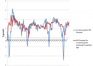
If this were easy to correct, macroeconomic forecasts would be much better. The following chart highlights the poor performance, however, of experts contributing to the quarterly Survey of Professional Forecasters, maintained by the Philadelphia Fed.

SPFcomp2

So, the red line is the SPF consensus forecast for GDP growth on a three quarter horizon, and the blue line is the forecast or nowcast for the current quarter (there is a delay in release of current numbers). Notice the huge dips in the current quarter estimate, associated with four recessions 1981, 1992, 2001-2, and 2008-9. A mere three months prior to these catastrophic drops in growth, leading forecasters at big banks, consulting companies, and universities totally missed the boat.

This is important in a practical sense, because recessions turn the world of many businesses upside down. All bets are off. The forecasting team is reassigned or let go as an economy measure, and so forth.

Some forward-looking information would help business intelligence focus on reallocating resources to sustain revenue as much as possible, using analytics to design cuts exerting the smallest impact on future ability to maintain and increase market share.

Hedgehogs and Foxes

Nate Silver has a great table in his best-selling The
Signal and the Noise
on the qualities and forecasting performance of hedgehogs and foxes. The idea comes from a Greek poet, “The fox knows many little things, but the hedgehog knows one big thing.”

Following Tetlock, Silver finds foxes are multidisplinary, adaptable, self-critical, cautious, and empirical, tolerant of complexity. By contrast, the Hedgehog is specialized, sticks to the same approaches, stubbornly adheres to his model in spite of counter-evidence, is order-seeking, confident, and ideological. The evidence suggests foxes generally outperform hedgehogs, just as ensemble methods typically outperform a single technique in forecasting.

Message – be a fox.

So maybe this can explain some of the breadth of this blog. If we have trouble predicting GDP growth, what about forecasts in other areas – such as weather, climate change, or that old chestnut, sun spots? And maybe it is useful to take a look at how to forecast all the inputs and associated series – such as exchange rates, growth by global region, the housing market, interest rates, as well as profits.

And while we are looking around, how about brain waves? Can brain waves be forecast? Oh yes, it turns out there is a fascinating and currently applied new approach called neuromarketing, which uses headbands and electrodes, and even MRI machines, to detect deep responses of consumers to new products and advertising.

New Methods

I know I have not touched on cluster analysis and classification, areas making big contributions to improvement of business process. But maybe if we consider the range of “new” techniques for predictive analytics, we can see time series forecasting and analysis of customer behavior coming under one roof.

There is, for example, this many predictor thread emerging in forecasting in the late 1990’s and especially in the last decade with factor models for macroeconomic forecasting. Reading this literature, I’ve become aware of methods for mapping N explanatory variables onto a target variable, when there are M<N observations. These are sometimes called methods of data shrinkage, and include principal components regression, ridge regression, and the lasso. There are several others, and a good reference is The Elements of Statistical Learning, Data Mining, Learning and Prediction, 2nd edition, by Trevor Hastie, Robert Tibshirani, and Jerome Friedman. This excellent text is downloadable, accessible via the Tools, Apps, Texts, Free Stuff menu option located just to the left of the search utility on the heading for this blog.

There also is bagging, which is the topic of the previous post, as well as boosting, and a range of decision tree and regression tree modeling tactics, including random forests.

I’m actively exploring a number of these approaches, ginning up little examples to see how they work and how the computation goes. So far, it’s impressive. This stuff can really improve over the old approaches, which someone pointed out, have been around since the 1950’s at least.

It’s here I think that we can sight the on-coming wave, just out there on the horizon – perhaps hundreds of feet high. It’s going to swamp the old approaches, changing market research forever and opening new vistas, I think, for forecasting, as traditionally understood.

I hope to be able to ride that wave, and now I put it that way, I get a sense of urgency in keeping practicing my web surfing.

Hope you come back and participate in the comments section, or email me at [email protected]

Forecasting in Data-limited Situations – A New Day

Over the Holidays – while frustrated in posting by a software glitch – I looked at the whole “shallow data issue” in light of  a new technique I’ve learned called bagging.

Bottom line, using spreadsheet simulations, I can show bagging radically reduces out-of-sample forecast error, in a situation typical for a lot business forecasting – where there are just a few workable observations, quite a few candidate drivers or explanatory variables, and a lot of noise in the data.

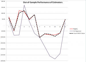
Here is a comparison of the performance of OLS regression and bagging with out-of-sample data generated with the same rules which create the “sample data” in the example spreadsheet shown below.

SmallDATAgraphcomp

The contrast is truly stark. Although, as we will see, the ordinary least squares (OLS) regression has an R2 or “goodness of fit” of 0.99, it does not generalize well out-of-sample, producing the purple line in the graph with 12 additional cases or observations. Bagging the original sample 200 times and re-estimating OLS regression on the bagged samples, then averaging the regression constants and coefficients, produces a much tighter fit on these out-of-sample observations.

Example Spreadsheet

The spreadsheet below illustrates 12 “observations” on a  TARGET or dependent variable and nine (9) explanatory variables, x1 through x9.

SmallDATA1

The top row with numbers in red lists the “true” values of these explanatory variables or drivers, and the column of numbers in red on the far right are the error terms (which are generated by a normal distribution with zero mean and standard deviation of 50).

So if we multiply 3 times 0.22 and add -6 times -2.79 and so forth, adding 68.68 at the end, we get the first value of the TARGET variable 60.17.

While this example is purely artificial, an artifact, one can imagine that these numbers are first differences – that is the current value of a variable minus its preceding value. Thus, the TARGET variable might record first differences in sales of a product quarter by quarter. And we suppose forecasts for  x1 through x9 are available, although not shown above. In fact, they are generated in simulations with the same generating mechanisms utilized to create the sample.

Using the simplest multivariate approach, the ordinary least squares (OLS) regression, displayed in the Excel format, is –

SmallDATAreg

There’s useful information in this display, often the basis of a sort of “talk-through” the regression result. Usually, the R2 is highlighted, and it is terrific here, “explaining” 99 percent of the variation in the data, in, that is, the 12 in-sample values for the TARGET variable. Furthermore, four explanatory variables have statistically significant coefficients, judged by their t-statistics – x2, x6, x7, and x9. These are highlighted in a kind of purple in the display.

Of course, the estimated values of x1 through x9 are, for the most part, numerically quite different than the true values of the constant term and coefficients {10, 3, -6, 0.5, 15, 1, -1, -5, 0.25, 1}. Nevertheless, because of the large variances or standard errors of the estimates, as noted above some estimated coefficients are within a 95 percent confidence interval of these true values. It’s just that the confidence intervals are very wide.

The in-sample predicted values are accurate, generally speaking. These loopy coefficient estimates essentially balance one another off in-sample.

But it’s not the in-sample performance we are interested in, but the out-of-sample performance. And we want to compare the out-of-sample performance of this OLS regression estimate with estimates of the coefficients and TARGET variable produced by ridge regression and bagging.

Bagging

Bagging [bootstrap aggregating] was introduced by Breiman in the 1990’s to reduce the variance of predictors. The idea is that you take N bootstrap samples of the original data, and with each of these samples, estimate your model, creating, in the end, an ensemble prediction.

Bootstrap sampling draws random samples with replacement from the original sample, creating other samples of the same size. With 12 cases or observations on the TARGET and explanatory variables there are a large number of possible random samples of these 12 cases drawn with replacement; in fact, given nine explanatory variables and the TARGET variable, there are 129  or somewhat more than 5 billion distinct samples, 12 of which, incidentally, are comprised of exactly the same case drawn repeatedly from the original sample.

A primary application of bagging has been in improving the performance of decision trees and systems of classification. Applications to regression analysis seem to be more or less an after-thought in the literature, and the technique does not seem to be in much use in applied business forecasting contexts.

Thus, in the spreadsheet above, random draws with replacement are taken of the twelve rows of the spreadsheet (TARGET and drivers) 200 times, creating 200 samples. An ordinary least squares regression is estimated over each regression, and the constant and parameter estimates are averaged at the end of the process.

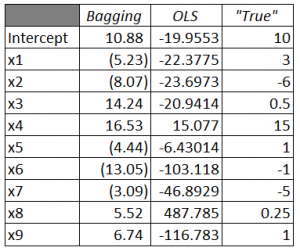
Here is a comparison of the estimated coefficients from Bagging and OLS, compared with the true values.

BaggingTable

There’s still variation of the parameter estimates from the true values with bagging, but the variance of the error process (50) is, by design, high. For example, most of the value of TARGET is from the error process, so this is noisy data.

Discussion

Some questions. For example – Are there specific features of the problem presented here which tip the results markedly in favor of bagging? What are the criteria for determining whether bagging will improve regression forecasts? Another question regards the ease or difficulty of bagging regressions in Excel.

The criterion for bagging to deliver dividends is basically parameter instability over the sample. Thus, in the problem here, deleting any observation from the 12 cases and re-estimating the regression results in big changes to estimated parameters. The basic reason is the error terms constitute by far the largest contribution to the value of TARGET for each case.

In practical forecasting, this criterion, which not very clearly defined, can be explored, and then comparisons with regard to actual outcomes can be studied. Thus, estimate the bagged regression forecast,  wait a period, and compare bagged and simple OLS forecasts. Substantial improvement in forecast accuracy, combined with parameter instability in the sample, would seem to be a smoking gun.

Apart from the large contribution of the errors or residuals to the values of TARGET, the other distinctive feature of the problem presented here is the large number of predictors in comparison with the number of cases or observations. This, in part, accounts for the high coefficient of determination or R2, and also suggests that the close in-sample fit and poor out-of-sample performance are probably related to “over-fitting.”