Tag Archives: stock market forecasts

One-Month-Ahead Stock Market Forecasts

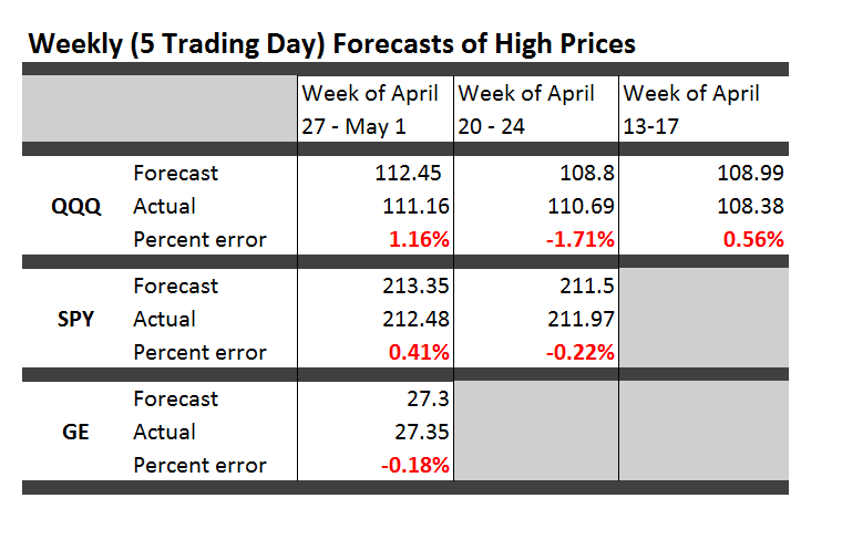
I have been spending a lot of time analyzing stock market forecast algorithms I stumbled on several months ago which I call the New Proximity Algorithms (NPA’s).

There is a white paper on the University of Munich archive called Predictability of the Daily High and Low of the S&P 500 Index. This provides a snapshot of the NPA at one stage of development, and is rock solid in terms of replicability. For example, an analyst replicated my results with Python, and I’ll probably will provide his code here at some point.

I now have moved on to longer forecast periods and more complex models, and today want to discuss month-ahead forecasts of high and low prices of the S&P 500 for this month – June.

Current Month Forecast for S&P 500

For the current month – June 2015 – things look steady with no topping out or crash in sight

With opening price data from June 1, the NPA month-ahead forecast indicates a high of 2144 and a low of 2030. These are slightly above the high and low for May 2015, 2,134.72 and 2,067.93, respectively.

But, of course, a week of data for June already is in, so, strictly speaking, we need a three week forecast, rather than a forecast for a full month ahead, to be sure of things. And, so far, during June, daily high and low prices have approached the predicted values, already.

In the interests of gaining better understanding of the model, however, I am going to “talk this out” without further computations at this moment.

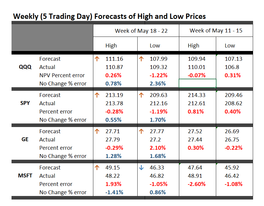
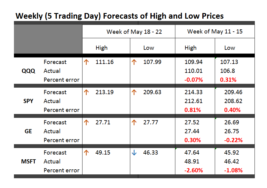
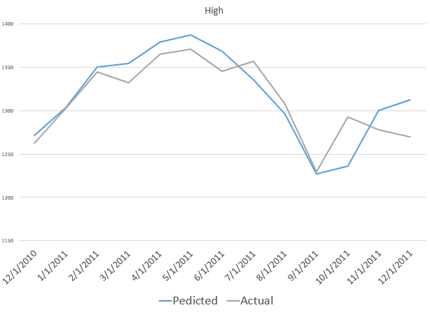
So, one point is that the model for the low is less reliable than the high price forecast on a month-ahead basis. Here, for example, is the track record of the NPA month-ahead forecasts for the past 12 months or so with S&P 500 data.

12MOSNPA

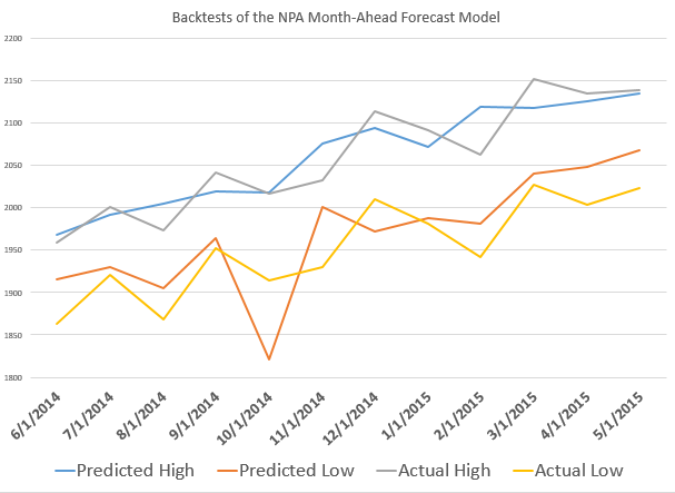
The forecast model for the high tracks along with the actuals within around 1 percent forecast error, plus or minus. The forecast model for the low, however, has a big miss with around 7 percent forecast error in late 2014.

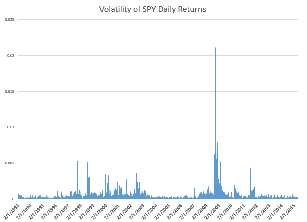
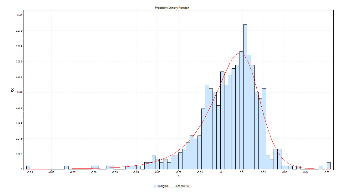
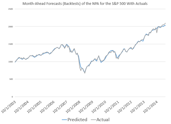
This sort of “wobble” for the NPA forecast of low prices is not unusual, as the following chart, showing backtests to 2003, shows.

LowMonthAheadBig

What’s encouraging is the NPA model for the low price adjusts quickly. If large errors signal a new direction in price movement, the model catches that quickly. More often, the wobble in the actual low prices seems to be transitory.

Predicting Turning Points

One reason why the NPA monthly forecast for June might be significant, is that the underlying method does a good job of predicting major turning points.

If a crash were coming in June, it seems likely, based on backtesting, that the model would signal something more than a slight upward trend in both the high and low prices.

Here are some examples.

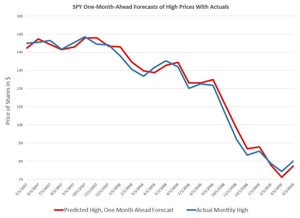
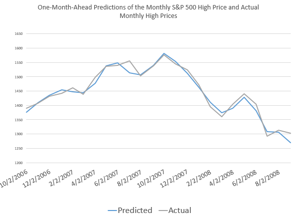
First, the NPA forecast model for the high price of the S&P 500 caught the turning point in 2007 when the market began to go into reverse.

S&P2008high

But that is not all.

The NPA model for the month-ahead high price also captures a more recent reversal in the S&P 500.

laterHighS&P500


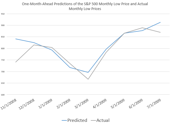
Also, the model for the low did capture the bottom in the S&P 500 in 2009, when the direction of the market changed from decline to increase.

2008High

This type of accuracy in timing in forecast modeling is quite remarkable.

It’s something I also saw earlier with the Hong Kong Hang Seng Index, but which seemed at that stage of model development to be confined to Chinese market data.

Now I am confident the NPA forecasts have some capability to predict turning points quite widely across many major indexes, ETF’s, and markets.

Note that all the charts shown above are based on out-of-sample extrapolations of the NPA model. In other words, one set of historical data are used to estimate the parameters of the NPA model, and other data, outside this sample, are then plugged in to get the month-ahead forecasts of the high and low prices.

Where This Is Going

I am compiling materials for presentations relating to the NPA, its capabilities, its forecast accuracy.

The NPA forecasts, as the above exhibits show, work well when markets are going down or turning directions, as when in a steady period of trending growth.

But don’t mistake my focus on these stock market forecasting algorithms for a last minute conversion to the view that nothing but the market is important. In fact, a lot of signals from business and global data suggest we could be in store for some big changes later in 2015 or in 2016.

What I want to do, I think, is understand how stock markets function as sort of prisms for these external developments – perhaps involving Greek withdrawal from the Eurozone, major geopolitical shifts affecting oil prices, and the onset of the crazy political season in the US.

Multivariate GARCH and Portfolio Risk Management

Why get involved with the complexity of multivariate GARCH models?

Well, because you may want to exploit systematic and persisting changes in the correlations of stocks and bonds, and other major classes of financial assets. If you know how these correlations change over, say, a forecast horizon of one month, you can do a better job of balancing risk in portfolios.

This a lively area of applied forecasting, as I discovered recently from Henry Bee of Cassia Research – based in Vancouver, British Columbia (and affiliated with CONCERT Capital Management of San Jose, California). Cassia Research provides Institutional Quant Technology for Investment Advisors.

HenryBee

Basic Idea The key idea is that the volatility of stock prices cluster in time, and most definitely is not a random walk. Just to underline this – volatility is classically measured as the square of daily stock returns. It’s absolutely straight-forward to make a calculation and show that volatility clusters, as for example with this more than year series for the SPY exchange traded fund.

SPYVolatility

Then, if you consider a range of assets, calculating not only their daily volatilities, in terms of their own prices, but how these prices covary – you will find similar clustering of covariances.

Multivariate GARCH models provide an integrated solution for fitting and predicting these variances and covariances. For a key survey article, check out – Multivariate GARCH Models A Survey.

Some quotes from the company site provide details: We use a high-frequency multivariate GARCH model to control for volatility clustering and spillover effects, reducing drawdowns by 50% vs. historical variance. …We are able to tailor our systems to target client risk preferences and stay within their tolerance levels in any market condition…. [Dynamic Rebalancing can]..adapt quickly to market shifts and reduce drawdowns by dynamically changing rebalance frequency based on market behavior.

The COO of Cassia Research also is a younger guy – Jesse Chen. As I understand it, Jesse handles a lot of the hands-on programming for computations and is the COO.

JesseChen

I asked Bee what he saw as the direction of stock market and investment volatility currently, and got a surprising answer. He pointed me to the following exhibit on the company site.

Bee1 The point is that for most assets considered in one of the main portfolios targeted by Cassia Research, volatilities have been dropping – as indicated by the negative signs in the chart. These are volatilities projected ahead by one month, developed by the proprietary multivariate GARCH modeling of this company – an approach which exploits intraday data for additional accuracy.

There is a wonderful 2013 article by Kirilenko and Lo called Moore’s Law versus Murphy’s Law: Algorithmic Trading and Its Discontents. Look on Google Scholar for this title and you will find a downloadable PDF file from MIT.

The Quant revolution in financial analysis is here to stay, and, if you pay attention, provides many examples of successful application of forecasting algorithms.

Stock Market Price Predictability, Random Walks, and Market Efficiency

Can stock market prices be predicted? Can they be predicted with enough strength to make profits?

The current wisdom may be that market predictability is like craps. That is, you might win (correctly predict) for a while, maybe walking away with nice winnings, if you are lucky. But over the long haul, the casino is the winner.

This seems close to the view in Andrew P. Lo and Craig MacKinlay’s A NonRandom Walk Down Wall Street (NRW), a foil to Burton Malkiel’s A Random Walk Down Wall Street, perhaps.

Lo and MacKinlay (L&M) collect articles from the 1980’s and 1990’s – originally published in the “very best journals” – in a 2014 compilation with interesting intoductions and discussions.

Their work more or less conclusively demonstrates that US stock market prices are not, for identified historic periods, random walks.

The opposite idea – that stock prices are basically random walks – has a long history, “recently” traceable to the likes of Paul Samuelson, as well as Burton Malkiel. Supposedly, any profit opportunity in a deeply traded market will be quickly exploited, leaving price movements largely random.

The ringer for me in this whole argument is the autocorrelation (AC) coefficient.

The first order autocorrelation coefficient of a random walk is 1, but metrics derived from stock price series have positive first order autocorrelations less than 1 over daily or weekly data. In fact, L&M were amazed to discover the first order autocorrelation coefficient of weekly stock returns, based on CRSP data, was 30 percent and statistically highly significant. In terms of technical approach, a key part of their analysis involves derivation of asymptotic limits for distributions and confidence intervals, based on assumptions which encompass nonconstant (heteroskedastic) error processes.

Finding this strong autocorrelation was somewhat incidental to their initial attack on the issue of the randomness, which is based on variance ratios.

L&M were really surprised to discover significant AC in stock market returns, and, indeed, several of their articles explore ways they could be wrong, or things could be different than what they appear to be.

All this is more than purely theoretical, as Morgan Stanley and D.P. Shaw’s development of “high frequency equity trading strategies” shows. These strategies exploit this autocorrelation or time dependency through “statistical arbitrage.” By now, though, according to the authors, this is a thin-margin business, because of the “proliferation of hedge funds engaged in these activities.”

Well, there are some great, geeky lines for cocktail party banter, such as “rational expectations equilibrium prices need not even form a martingale sequence, of which the random walk is special case.”

By itself, the “efficient market hypothesis” (EFM) is rather nebulous, and additional contextualization is necessary to “test” the concept. This means testing several joint hypotheses. Accordingly, negative results can simply be attributed to failure of one or more collateral assumptions. This builds a protective barrier around the EFM, allowing it to retain its character as an article of faith among many economists.

AWL

Andrew W. Lo is a Professor of Finance at MIT and Director of the Laboratory for Financial Engineering. His site through MIT lists other recent publications, and I would like to draw readers’ attention to two:

Can Financial Engineering Cure Cancer?

Reading About the Financial Crisis: A Twenty-One-Book Review

Thoughts on Stock Market Forecasting

Here is an update on the forecasts from last Monday – forecasts of the high and low of SPY, QQQ, GE, and MSFT.

This table is easy to read, even though it is a little” busy”.

TableMay22

One key is to look at the numbers highlighted in red and blue (click to enlarge).

These are the errors from the week’s forecast based on the NPV algorithm (explained further below) and a No Change forecast.

So if you tried to forecast the high for the week to come, based on nothing more than the high achieved last week – you would be using a No Change model. This is a benchmark in many forecasting discussions, since it is optimal (subject to some qualifications) for a random walk. Of course, the idea stock prices are a random walk came into favor several decades ago, and now gradually is being rejected of modified, based on findings such as those above.

The NPV forecasts are more accurate for this last week than No Change projections 62.5 percent of the time, or in 5 out of the 8 forecasts in the table for the week of May 18-22. Furthermore, in all three cases in which the No Change forecasts were better, the NPV forecast error was roughly comparable in absolute size. On the other hand, there were big relative differences in the absolute size of errors in the situations in which the NPV forecasts proved more accurate, for what that is worth.

The NPV algorithm, by the way, deploys various price ratios (nearby prices) and their transformations as predictors. Originally, the approach focused on ratios of the opening price in a period and the high or low prices in the previous period. The word “new” indicates a generalization has been made from this original specification.

Ridge Regression

I have been struggling with Visual Basic and various matrix programming code for ridge regression with the NPV specifications.

Using cross validation of the λ parameter, ridge regression can improve forecast accuracy on the order of 5 to 10 percent. For forecasts of the low prices, this brings forecast errors closer to acceptable error ranges.

Having shown this, however, I am now obligated to deploy ridge regression in several of the forecasts I provide for a week or perhaps a month ahead.

This requires additional programming to be convenient and transparent to validation.

So, I plan to work on that this coming week, delaying other tables with weekly or maybe monthly forecasts for a week or so.

I will post further during the coming week, however, on the work of Andrew Lo (MIT Financial Engineering Center) and high frequency data sources in business forecasts.

Probable Basis of Success of NPV Forecasts

Suppose you are an observer of a market in which securities are traded. Initially, tests show strong evidence stock prices in this market follow random walk processes.

Then, someone comes along with a theory that certain price ratios provide a guide to when stock prices will move higher.

Furthermore, by accident, that configuration of price ratios occurs and is associated with higher prices at some date, or maybe a couple dates in succession.

Subsequently, whenever price ratios fall into this configuration, traders pile into a stock, anticipating its price will rise during the next trading day or trading period.

Question – isn’t this entirely plausible, and would it not be an example of a self-confirming prediction?

I have a draft paper pulling together evidence for this, and have shared some findings in previous posts. For example, take a look at the weird mirror symmetry of the forecast errors for the high and low.

And, I suspect, the absence or ambivalence of this underlying dynamic is why closing prices are harder to predict than period high or low prices of a stock. If I tell you the closing price will be higher, you do not necessarily buy the stock. Instead, you might sell it, since the next morning opening prices could jump down. Or there are other possibilities.

Of course, there are all kinds of systems traders employ to decide whether to buy or sell a stock, so you have to cast your net pretty widely to capture effects of the main methods.

Long Term Versus Short Term

I am getting mixed results about extending the NPV approach to longer forecast horizons – like a quarter or a year or more.

Essentially, it looks to me as if the No Change model becomes harder and harder to beat over longer forecast horizons – although there may be long run persistence in returns or other features that I see  other researchers (such as Andrew Lo) have noted.

Monday Morning Stock Forecasts May 18 – Highs and Lows for SPY, QQQ, GE, and MSFT

Look at it this way. There are lots of business and finance blogs, but how many provide real-time forecasts, along with updates on how prior predictions performed?

Here on BusinessForecastBlog – we roll out forecasts of the highs and lows of a growing list of securities for the coming week on Monday morning, along with an update on past performance.

It’s a good discipline, if you think you have discovered a pattern which captures some part of the variation in future values of a variable. Do the backtesting, but also predict in real-time. It’s very unforgiving.

Here is today’s forecast, along with a recap for last week (click to enlarge).TableMay18

There is an inevitable tendency to narrate these in “Nightly Business Report” fashion.

So the highs are going higher this week, and so are the lows, except perhaps for a slight drop in Microsoft’s low – almost within the margin of statistical noise. Not only that, but predicted increases in the high for QQQ are fairly substantial.

Last week’s forecasts were solid, in terms of forecast error, except Microsoft’s high came in above what was forecast. Still, -2.6 percent error is within the range of variation in the backtests for this security. Recall, too, that in the previous week, the forecast error for the high of MSFT was only .04 percent, almost spot on.

Since the market moved sideways for many securities, No Change forecasts were a strong competitor to the NPV (new proximity variable) forecasts. In fact, there was an 50:50 split. In half the four cases, the NPV forecasts performed better; in the other half, No Change forecasts had lower errors.

Direction of change predictions also came in about 50:50. They were correct for QQQ and SPY, and wrong for the two stocks.

Where is the Market Going?

This tool – forecasts based on the NPV algorithms – provides longer terms looks into the future, probably effectively up to one month ahead.

So in two weeks, I’m going to add that forecast to the mix. I think it may be important, incidentally, to conform to the standard practice of taking stock at the beginning of the month, rather than, say, simply going out four weeks from today.

To preview the power of this monthly NPV model, here are the backtests for the crisis months before and during the 2008 financial crisis.

SPYM2008

This is a remarkable performance, really. Once the crash really gets underway in late Summer-Fall 2008, the NPV forecast drops in a straight-line descent, as do the actual monthly highs. There are some turning points in common, too, between the two series. And generally, even at the start of the process, the monthly NPV model provides good guidance as to the direction and magnitude of changes.

Over the next two weeks, I’m collecting high frequency data to see whether I can improve these forecasts with supplemental information – such as interest rates spreads and other variables available on a weekly or monthly basis.

In closing, let me plug Barry Eichengreen’s article in Syndicate An Economics to Fit the Facts.

Eichengreen writes,

While older members of the economics establishment continue to debate the merits of competing analytical frameworks, younger economists are bringing to bear important new evidence about how the economy operates.

It’s all about dealing with the wealth of data that is being collected everywhere now, and much less about theoretical disputes involving formal models.

Finally, it’s always necessary to insert a disclaimer, whenever one provides real-time, actionable forecasts. This stuff is for informational and scientific purposes only. It is not intended to provide recommendations for specific stock trading, and what you do on that score is strictly your own business and responsibility.

Mountain climbing pic from Blink.

Reading the Tea Leaves – Forecasts of Stock High and Low Prices

The residuals of predictive models are central to their statistical evaluation – with implications for confidence intervals of forecasts.

Of course, another name for the residuals of a predictive model is their errors.

Today, I want to present some information on the errors for the forecast models that underpin the Monday morning forecasts in this blog.

The results are both reassuring and challenging.

The good news is that the best fit distributions support confidence intervals, and, in some cases, can be viewed as transformations of normal variates. This is by no means given, as monstrous forms such as the Cauchy distribution sometimes present themselves in financial modeling as a best candidate fit.

The challenge is that the skew patterns of the forecasts of the high and low prices are weirdly symmetric. It looks to me as if traders tend to pile on when the price signals are positive for the high, or flee the sinking ship when the price history indicates the low is going lower.

Here is the error distribution of percent errors for backtests of the five day forecast of the QQQ high, based on an out-of-sample study from 2004 to the present, a total of 573 five consecutive trading day periods.

JohnSUHigh

Here is the error distribution of percent errors for backtests of the five day forecast of the QQQ low.

JohnSULow

In the first chart for forecasts of high prices, errors are concentrated in the positive side of the percent error or horizontal axis. In the second graph, errors from forecasts of low prices are concentrated on the negative side of the horizontal axis.

In terms of statistics-speak, the first chart is skewed to the left, having a long tail of values to the left, while the second chart is skewed to the right.

What does this mean? Well, one interpretation is that traders are overshooting the price signals indicating a positive change in the high price or a lower low price.

Thus, the percent error is calculated as

(Actual – Predicted)/Actual

So the distribution of errors for forecasts of the high has an average which is slightly greater than zero, and the average for errors for forecasts of the low is slightly negative. And you can see the bulk of observations being concentrated, on the one hand, to the right of zero and, on the other, to the left of zero.

I’d like to find some way to fill out this interpretation, since it supports the idea that forecasts in this context are self-reinforcing, rather than self-nihilating.

I have more evidence consistent with this interpretation. So, if traders dive in when prices point to a high going higher, predictions of the high should be more reliable vis a vis direction of change with bigger predicted increases in the high. That’s also verifiable with backtests.

I use MathWave’s EasyFit. It’s user-friendly, and ranks best fit distributions based on three standard metrics of goodness of fit – the Chi-Squared, Komogorov-Smirnov, and Anderson-Darling statistics. There is a trial download of the software, if you are interested.

The Johnson SU distribution ranks first for the error distribution for the high forecasts, in terms of EasyFit’s measures of goodness of fit. The Johnson SU distribution also ranks first for Chi-Squared and the Anderson-Darling statistics for the errors of forecasts of the low.

This is an interesting distribution which can be viewed as a transformation of normal variates and which has applications, apparently, in finance (See http://www.ntrand.com/johnson-su-distribution/).

It is something I have encountered repeatedly in analyzing errors of proximity variable models. I am beginning to think it provides the best answer in determining confidence intervals of the forecasts.

Top picture from mysteryarts


Five Day Forecasts of High and Low for QQQ, SPY, GE, and MSFT – Week of May 11-15

Here are high and low forecasts for two heavily traded exchange traded funds (ETF’s) and two popular stocks. Like the ones in preceding weeks, these are for the next five trading days, in this case Monday through Friday May 11-15.

HLWeekMay11to15

The up and down arrows indicate the direction of change from last week – for the high prices only, since the predictions of lows are a new feature this week.

Generally, these prices are essentially “moving sideways” or with relatively small changes, except in the case of SPY.

For the record, here is the performance of previous forecasts.

TableMay8

Strong disclaimer: These forecasts are provided for information and scientific purposes only. This blog accepts no responsibility for what might happen, if you base investment or trading decisions on these forecasts. What you do with these predictions is strictly your own business.

Incidentally, let me plug the recent book by Andrew W. Lo and A. Craig McKinlay – A Non-Random Walk Down Wall Street from Princeton University Press and available as a e-book.

I’ve been reading an earlier book which Andrew Lo co-authored The Econometrics of Financial Markets.

What I especially like in these works is the insistence that statistically significant autocorrelations exist in stock prices and stock returns. They also present multiple instances in which stock prices fail tests for being random walks, and establish a degree of predictability for these time series.

Again, almost all the focus of work in the econometrics of financial markets is on closing prices and stock returns, rather than predictions of the high and low prices for periods.

How Did This Week’s Forecasts of QQQ, SPY, GE, and MSFT High Prices Do?

The following Table provides an update for this week’s forecasts of weekly highs for the securities currently being followed – QQQ, SPY, GE, and MSFT. Price forecasts and actual numbers are in US dollars.

TableMay8

This batch of forecasts performed extremely well in terms of absolute size of forecast errors, and, in addition, beating a “no change” forecast in three out of four predictions (exception being SPY) and correctly calling the change in direction of the high for QQQ.

It would be nice to be able to forecast the high prices for five-day-forward periods with the accuracy seen in the Microsoft (MSFT) forecast.

As all you market mavens know, US stock markets experienced a lot of declines in prices this week, so the highs for the week occurred Monday.

I’ve had several questions about the future direction of the market. Are declines going to be in the picture for the coming week, and even longer, for example?

I’ve been studying the capabilities of these algorithms to predict turning points in indexes and prices of individual securities. The answer is going to be probabilistic, and so is complicated. Sometimes the algorithm seems to provide pretty unambiguous signals as to turning points. In other instances, the tea leaves are harder to read, but, arguably, a signal does exist for most major turning points with the indexes I have focused on – SPY, QQQ, and the S&P 500.

So, the next question is – has the market hit a high for a week or a few weeks, or even perhaps a major turnaround?

Deploying these algorithms, coded in Visual Basic and C#, to attack this question is a little like moving a siege engine to the castle wall. A major undertaking.

I want to get there, but don’t want to be a “Chicken Little” saying “the sky is falling,” “the sky is falling.”

Stock Market Predictability

This little Monday morning exercise, which will be continued for the next several weeks, is providing evidence for the predictability of aspects of stock prices on a short term basis.

Once the basic facts are out there for everyone to see, a lot of questions arise. So what about new information? Surely yesterday’s open, high, low, and closing prices, along with similar information for previous days, do not encode an event like 9/11, or the revelation of massive accounting fraud with a stock issuing concern.

But apart from such surprises, I’m leaning to the notion that a lot more information about the general economy, company prospects and performance, and so forth are subtly embedded in the flow of price data.

I talked recently with an analyst who is applying methods from Kelly and Pruitt’s Market Expectations in the Cross Section of Present Values for wealth management clients. I hope to soon provide an “in-depth” on this type of applied stock market forecasting model, which focuses, incidentally, on stock market returns and dividends.

There is also some compelling research on the performance of momentum trading strategies which seems to indicate a higher level of predictability in stock prices than is commonly thought to exist.

Incidentally, in posting this slightly before the bell today, Friday, I am engaging in intra-day forecasting – betting that prices for these securities will stay below their earlier highs.

Forecasts of High Prices for Week May 4-8 – QQQ, SPY, GE, and MSFT

Here are forecasts of high prices for key securities for this week, May 4-8, along with updates to check the accuracy of previous forecasts. So far, there is a new security each week. This week it is Microsoft (MSFT). Click on the Table to enlarge.

TableMay4

These forecasts from the new proximity variable (NPV) algorithms compete with the “no change” forecast – supposedly the optimal predictions for a random walk.

The NPV forecasts in the Table are more accurate than no change forecasts at 3:2 odds. That is, if you take into account the highs of the previous weeks for each security – actual high numbers not shown in the Table – the NPV forecasts are more accurate 4 out of 6 times.

This performance corresponds roughly with the improvements of the NPV approach over the no change forecasts in backtests back to 2003.

The advantages of the NPV approach extend beyond raw accuracy, measured here in simple percent terms, since the “no change” forecast is uninformative about the direction of change. The NPV forecasts, on the other hand, generally get the direction of change right. In the Table above, again considering data from weeks preceding those shown, the direction of change of the high forecasts is spot on every time. Backtests suggest the NPV algorithm will correctly predict the direction of change of the high price about 75 percent of the time for this five day interval.

It will be interesting to watch QQQ in this batch of forecasts. This ETF is forecast to decline week-over-week in terms of the high price.

Next week I plan to expand the forecast table to include forecasts of the low prices.

There is a lot of information here. Much of the finance literature focuses on the rates of returns based on closing prices, or adjusted closing prices. Perhaps analysts figure that attempting to predict “extreme values” is not a promising idea. Nothing could be further from the truth.

This week I plan a post showing how to identify turning points in the movement of major indices with the NPV algorithms. The concept is simple. I forecast the high and low over coming periods, like a day, five days, ten trading days and so forth. For these “nested forecast periods” the high for the week ahead must be greater than or equal to the high for tomorrow or shorter periods. This means when the price of the SPY or QQQ heads south, the predictions of the high of these ETF’s sort of freeze at a constant value. The predictions for the low, however, plummet.

Really pretty straight-forward.

I’ve appreciated and benefitted from your questions, comments, and suggestions. Keep them coming.

Track Record of Forecasts of High Prices

Well, US markets have closed for the week, and here is an update on how our forecasts did.

TableMay1

Apart from the numbers, almost everything I wrote last Monday about market trends was wrong. Some of the highs were reached Monday, for example, and the market dived after that. The lowest forecast error is for GE, which backtesting suggests is harder to forecast than the SPY and QQQ.

I will keep doing this, expanding the securities covered for several weeks. I also hope to get smarter about using this tool.

Forecast Turning Points

I want to comment on how to use this approach to get forward information about turning points in the market.

While the research is on-going, the basic finding is that turning points, which we need to define as changes in the direction of a security or index which are sustained for several trading days or periods, are indicated by a simple tactic.

Suppose the QQQ reaches a high and then declines for several days or longer. Then, the forecasts of the high over 1, 2, and several days will tend to freeze at their initial or early values, while forecasts of low price over an expanding series of forecast periods will drop. There will, in other words, be a pronounced divergence between the forecasts of the high and low, when a turning point is in the picture.

There are interesting charts from 2008 highlighting these relationships between the high and low forecasts over telescoping forecast horizons.

I am fairly involved in some computer programming around this “proximity variable forecasting approach.” However, I am happy to dialogue with readers and interested parties via the Comments section in this blog. If you want to communicate off-line, send your email and what your interest or concern is.

And check the forecasts for this coming week, which I will have out Monday morning. Should be an interesting week.