Category Archives: random walk

Can stock market prices be predicted? Can they be predicted with enough strength to make profits?

The current wisdom may be that market predictability is like craps. That is, you might win (correctly predict) for a while, maybe walking away with nice winnings, if you are lucky. But over the long haul, the casino is the winner.

This seems close to the view in Andrew P. Lo and Craig MacKinlay’s A NonRandom Walk Down Wall Street (NRW), a foil to Burton Malkiel’s A Random Walk Down Wall Street, perhaps.

Lo and MacKinlay (L&M) collect articles from the 1980’s and 1990’s – originally published in the “very best journals” – in a 2014 compilation with interesting intoductions and discussions.

Their work more or less conclusively demonstrates that US stock market prices are not, for identified historic periods, random walks.

The opposite idea – that stock prices are basically random walks – has a long history, “recently” traceable to the likes of Paul Samuelson, as well as Burton Malkiel. Supposedly, any profit opportunity in a deeply traded market will be quickly exploited, leaving price movements largely random.

The ringer for me in this whole argument is the autocorrelation (AC) coefficient.

The first order autocorrelation coefficient of a random walk is 1, but metrics derived from stock price series have positive first order autocorrelations less than 1 over daily or weekly data. In fact, L&M were amazed to discover the first order autocorrelation coefficient of weekly stock returns, based on CRSP data, was 30 percent and statistically highly significant. In terms of technical approach, a key part of their analysis involves derivation of asymptotic limits for distributions and confidence intervals, based on assumptions which encompass nonconstant (heteroskedastic) error processes.

Finding this strong autocorrelation was somewhat incidental to their initial attack on the issue of the randomness, which is based on variance ratios.

L&M were really surprised to discover significant AC in stock market returns, and, indeed, several of their articles explore ways they could be wrong, or things could be different than what they appear to be.

All this is more than purely theoretical, as Morgan Stanley and D.P. Shaw’s development of “high frequency equity trading strategies” shows. These strategies exploit this autocorrelation or time dependency through “statistical arbitrage.” By now, though, according to the authors, this is a thin-margin business, because of the “proliferation of hedge funds engaged in these activities.”

Well, there are some great, geeky lines for cocktail party banter, such as “rational expectations equilibrium prices need not even form a martingale sequence, of which the random walk is special case.”

By itself, the “efficient market hypothesis” (EFM) is rather nebulous, and additional contextualization is necessary to “test” the concept. This means testing several joint hypotheses. Accordingly, negative results can simply be attributed to failure of one or more collateral assumptions. This builds a protective barrier around the EFM, allowing it to retain its character as an article of faith among many economists.

Andrew W. Lo is a Professor of Finance at MIT and Director of the Laboratory for Financial Engineering. His site through MIT lists other recent publications, and I would like to draw readers’ attention to two:

Can Financial Engineering Cure Cancer?

Reading About the Financial Crisis: A Twenty-One-Book Review

accuracy of forecasts, new proximity model, predictive analytics, random walk, stock market forecasts

Thoughts on Stock Market Forecasting

May 24, 2015 Clive Jones

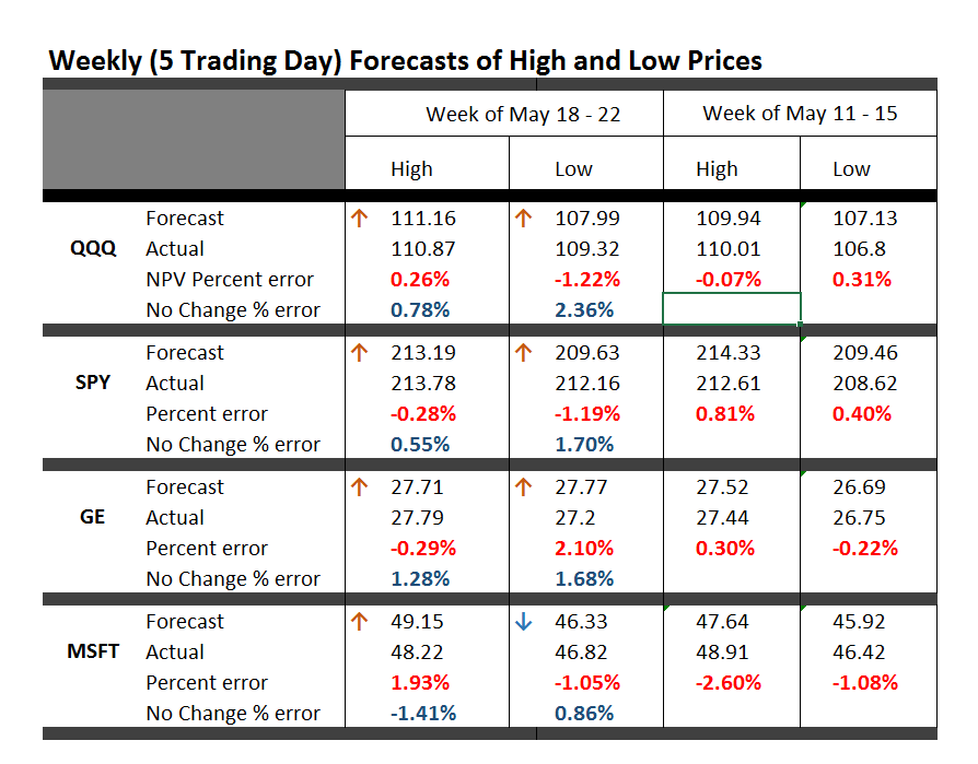
Here is an update on the forecasts from last Monday – forecasts of the high and low of SPY, QQQ, GE, and MSFT.

This table is easy to read, even though it is a little” busy”.

One key is to look at the numbers highlighted in red and blue (click to enlarge).

These are the errors from the week’s forecast based on the NPV algorithm (explained further below) and a No Change forecast.

So if you tried to forecast the high for the week to come, based on nothing more than the high achieved last week – you would be using a No Change model. This is a benchmark in many forecasting discussions, since it is optimal (subject to some qualifications) for a random walk. Of course, the idea stock prices are a random walk came into favor several decades ago, and now gradually is being rejected of modified, based on findings such as those above.

The NPV forecasts are more accurate for this last week than No Change projections 62.5 percent of the time, or in 5 out of the 8 forecasts in the table for the week of May 18-22. Furthermore, in all three cases in which the No Change forecasts were better, the NPV forecast error was roughly comparable in absolute size. On the other hand, there were big relative differences in the absolute size of errors in the situations in which the NPV forecasts proved more accurate, for what that is worth.

The NPV algorithm, by the way, deploys various price ratios (nearby prices) and their transformations as predictors. Originally, the approach focused on ratios of the opening price in a period and the high or low prices in the previous period. The word “new” indicates a generalization has been made from this original specification.

Ridge Regression

I have been struggling with Visual Basic and various matrix programming code for ridge regression with the NPV specifications.

Using cross validation of the λ parameter, ridge regression can improve forecast accuracy on the order of 5 to 10 percent. For forecasts of the low prices, this brings forecast errors closer to acceptable error ranges.

Having shown this, however, I am now obligated to deploy ridge regression in several of the forecasts I provide for a week or perhaps a month ahead.

This requires additional programming to be convenient and transparent to validation.

So, I plan to work on that this coming week, delaying other tables with weekly or maybe monthly forecasts for a week or so.

I will post further during the coming week, however, on the work of Andrew Lo (MIT Financial Engineering Center) and high frequency data sources in business forecasts.

Probable Basis of Success of NPV Forecasts

Suppose you are an observer of a market in which securities are traded. Initially, tests show strong evidence stock prices in this market follow random walk processes.

Then, someone comes along with a theory that certain price ratios provide a guide to when stock prices will move higher.

Furthermore, by accident, that configuration of price ratios occurs and is associated with higher prices at some date, or maybe a couple dates in succession.

Subsequently, whenever price ratios fall into this configuration, traders pile into a stock, anticipating its price will rise during the next trading day or trading period.

Question – isn’t this entirely plausible, and would it not be an example of a self-confirming prediction?

I have a draft paper pulling together evidence for this, and have shared some findings in previous posts. For example, take a look at the weird mirror symmetry of the forecast errors for the high and low.

And, I suspect, the absence or ambivalence of this underlying dynamic is why closing prices are harder to predict than period high or low prices of a stock. If I tell you the closing price will be higher, you do not necessarily buy the stock. Instead, you might sell it, since the next morning opening prices could jump down. Or there are other possibilities.

Of course, there are all kinds of systems traders employ to decide whether to buy or sell a stock, so you have to cast your net pretty widely to capture effects of the main methods.

Long Term Versus Short Term

I am getting mixed results about extending the NPV approach to longer forecast horizons – like a quarter or a year or more.

Essentially, it looks to me as if the No Change model becomes harder and harder to beat over longer forecast horizons – although there may be long run persistence in returns or other features that I see other researchers (such as Andrew Lo) have noted.

financial forecasting, predictive analytics, random walk, stock market forecasts, time series forecasting

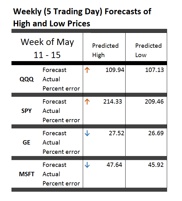
Five Day Forecasts of High and Low for QQQ, SPY, GE, and MSFT – Week of May 11-15

May 11, 2015 Clive Jones

Here are high and low forecasts for two heavily traded exchange traded funds (ETF’s) and two popular stocks. Like the ones in preceding weeks, these are for the next five trading days, in this case Monday through Friday May 11-15.

The up and down arrows indicate the direction of change from last week – for the high prices only, since the predictions of lows are a new feature this week.

Generally, these prices are essentially “moving sideways” or with relatively small changes, except in the case of SPY.

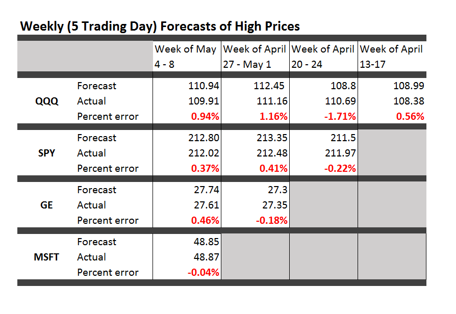
For the record, here is the performance of previous forecasts.

Strong disclaimer: These forecasts are provided for information and scientific purposes only. This blog accepts no responsibility for what might happen, if you base investment or trading decisions on these forecasts. What you do with these predictions is strictly your own business.

Incidentally, let me plug the recent book by Andrew W. Lo and A. Craig McKinlay – A Non-Random Walk Down Wall Street from Princeton University Press and available as a e-book.

I’ve been reading an earlier book which Andrew Lo co-authored The Econometrics of Financial Markets.

What I especially like in these works is the insistence that statistically significant autocorrelations exist in stock prices and stock returns. They also present multiple instances in which stock prices fail tests for being random walks, and establish a degree of predictability for these time series.

Again, almost all the focus of work in the econometrics of financial markets is on closing prices and stock returns, rather than predictions of the high and low prices for periods.

financial forecasts, predictive analytics, random walk, stock market forecasts

Some Comments on Forecasting High and Low Stock Prices

April 22, 2015 Clive Jones 1 Comment

I want to pay homage to Paul Erdős, the eccentric Hungarian-British-American-Israeli mathematician, whom I saw lecture a few years before his death. Erdős kept producing work in mathematics into his 70’s and 80’s – showing this is quite possible. Of course, he took amphetamines and slept on people’s couches while he was doing this work in combinatorics, number theory, and probability.

In any case, having invoked Erdős, let me offer comments on forecasting high and low stock prices – a topic which seems to be terra incognita, for the most part, to financial research.

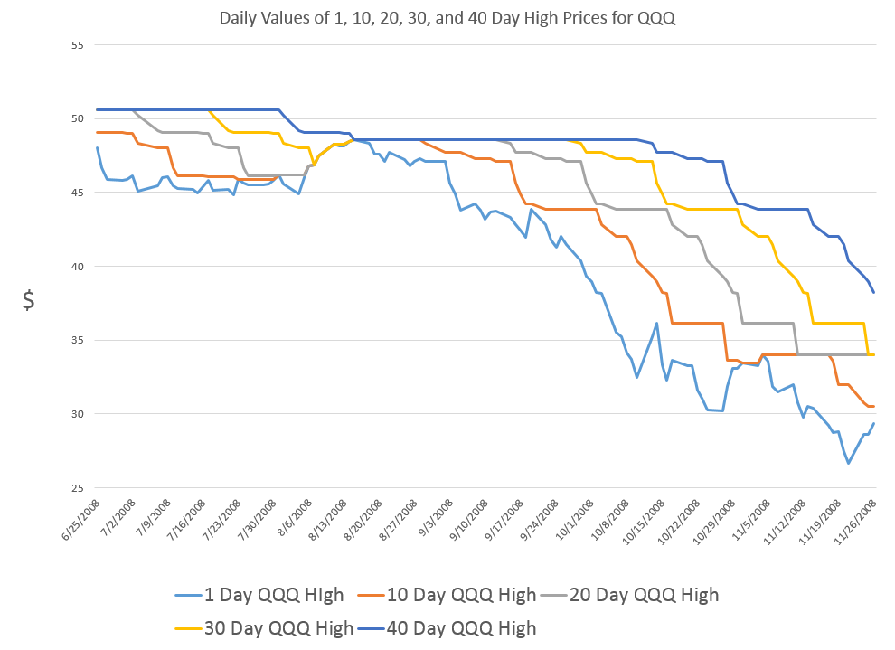
First, let’s take a quick look at a chart showing the maximum prices reached by the exchange traded fund QQQ over a critical period during the last major financial crisis in 2008-2009.

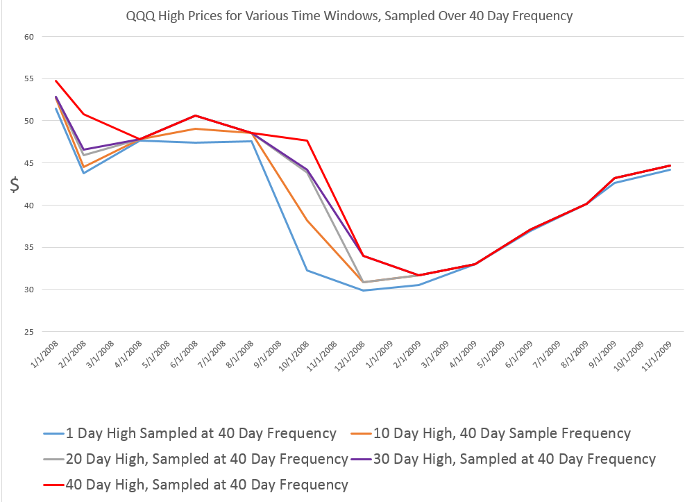
The graph charts five series representing QQQ high prices over periods extending from 1 day to 40 days.

The first thing to notice is that the variability of these time series decreases as the period for the high increases.

This suggests that forecasting the 40 day high could be easier than forecasting the high price for, say, tomorrow.

While this may be true in some sense, I want to point out that my research is really concerned with a slightly different problem.

This is forecasting ahead by the interval for the maximum prices. So, rather than a one-day-ahead forecast of the 40 day high price (which would include 39 known possible high prices), I forecast the high price which will be reached over the next 40 days.

This problem is better represented by the following chart.

This chart shows the high prices for QQQ over periods ranging from 1 to 40 days, sampled at what you might call “40 day frequencies.”

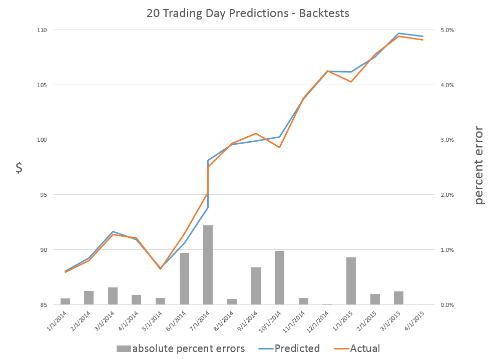
Now I am not quite going to 40 trading day ahead forecasts yet, but here are results for backtests of the algorithm which produces 20-trading-day-ahead predictions of the high for QQQ.

The blue lines shows the predictions for the QQQ high, and the orange line indicates the actual QQQ highs for these (non-overlapping) 20 trading day intervals. As you can see, the absolute percent errors – the grey bars – are almost all less than 1 percent error.

Random Walk

Now, these results are pretty good, and the question arises – what about the random walk hypothesis for stock prices?

Recall that a simple random walk can be expressed by the equation x_t=x_t-1 + ε_twhere ε_t is conventionally assumed to be distributed according to N(0,σ) or, in other words, as a normal distribution with zero mean and constant variance σ.

An interesting question is whether the maximum prices for a stock whose prices follow a random walk also can be described, mathematically, as a random walk.

This is elementary, when we consider that any two observations in a time series of random walks can be connected together as x_t+k = x_t + ω where ω is distributed according to a Gaussian distribution but does not necessarily have a constant variance for different values of the spacing parameter k.

From this it follows that the methods producing these predictions or forecasts of the high of QQQ over periods of several trading days also are strong evidence against the underlying QQQ series being a random walk, even one with heteroskedastic errors.

That is, I believe the predictability demonstrated for these series are more than cointegration relationships.

Where This is Going

While demonstrating the above point could really rock the foundations of finance theory, I’m more interested, for the moment, in exploring the extent of what you can do with these methods.

Very soon I’m going to post on how these methods may provide signals as to turning points in stock market prices.

Stay tuned, and thanks for your comments and questions.

Erdős picture from Encyclopaedia Britannica

ARIMA models, currency forecasts, financial forecasting, global business forecasts, gold price forecasting, predictive analytics, random walk

Forecasting the Price of Gold – 1

March 17, 2014 Clive Jones

I’m planning posts on forecasting the price of gold this week. This is an introductory post.

The Question of Price

What is the “price” of gold, or, rather, is there a single, integrated global gold market?

This is partly an anthropological question. Clearly in some locales, perhaps in rural India, people bring their gold jewelry to some local merchant or craftsman, and get widely varying prices. Presumably, though this merchant negotiates with a broker in a larger city of India, and trades at prices which converge to some global average. Very similar considerations apply to interest rates, which are significantly higher at pawnbrokers and so forth.

The World Gold Council uses the London PM fix, which at the time of this writing was $1,379 per troy ounce.

The Wikipedia article on gold fixing recounts the history of this twice daily price setting, dating back, with breaks for wars, to 1919.

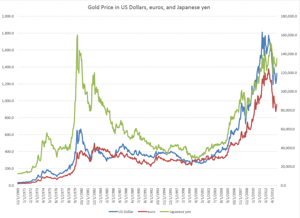
One thing is clear, however. The “price of gold” varies with the currency unit in which it is stated. The World Gold Council, for example, supplies extensive historical data upon registering with them. Here is a chart of the monthly gold prices based on the PM or afternoon fix, dating back to 1970.

Another insight from this chart is that the price of gold may be correlated with the price of oil, which also ramped up at the end of the 1970’s and again in 2007, recovering quickly from the Great Recession in 2008-09 to surge up again by 2010-11.

But that gets ahead of our story.

The Supply and Demand for Gold

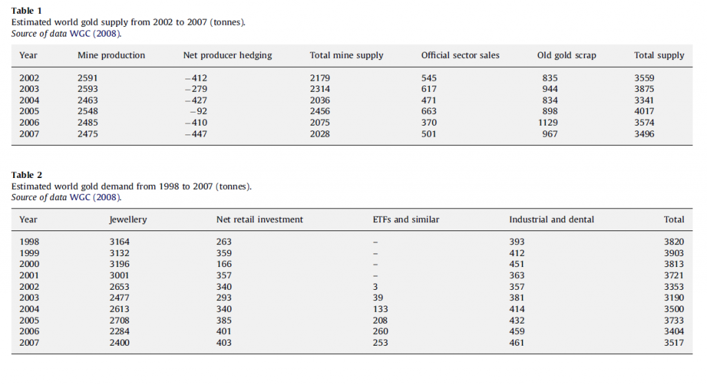
Here are two valuable tables on gold supply and demand fundamentals, based on World Gold Council sources, via an An overview of global gold market and gold price forecasting. I’ve more to say about the forecasting model in that article, but the descriptive material is helpful (click to enlarge).

These tables give an idea of the main components of gold supply and demand over a several years recently.

Gold is an unusual commodity in that one of its primary demand components – jewelry – can contribute to the supply-side. Thus, gold is in some sense renewable and recyclable.

Table 1 above shows the annual supplies in this period in the last decade ran on the order of three to four thousand tonnes, where a tonne is 2,240 pounds and equal conveniently to 1000 kilograms.

Demand for jewelry is a good proportion of this annual supply, with demands by ETF’s or exchange traded funds rising rapidly in this period. The industrial and dental demand is an order of magnitude lower and steady.

One of the basic distinctions is between the monetary versus nonmonetary uses or demands for gold.

In total, central banks held about 30,000 tonnes of gold as reserves in 2008.

Another estimated 30,000 tonnes was held in inventory for industrial uses, with a whopping 100,000 tonnes being held as jewelry.

India and China constitute the largest single countries in terms of consumer holdings of gold, where it clearly functions as a store of value and hedge against uncertainty.

Gold Market Activity

In addition to actual purchases of gold, there are gold futures. The CME Group hosts a website with gold future listings. The site states,

Gold futures are hedging tools for commercial producers and users of gold. They also provide global gold price discovery and opportunities for portfolio diversification. In addition, they: Offer ongoing trading opportunities, since gold prices respond quickly to political and economic events, Serve as an alternative to investing in gold bullion, coins, and mining stocks

Some of these contracts are recorded at exchanges, but it seems the bulk of them are over-the-counter.

A study by the London Bullion Market Association estimates that 10.9bn ounces of gold, worth $15,200bn, changed hands in the first quarter of 2011 just in London’s markets. That’s 125 times the annual output of the world’s gold mines – and twice the quantity of gold that has ever been mined.

The Forecasting Problem

The forecasting problem for gold prices, accordingly, is complex. Extant series for gold prices do exist and underpin a lot of the market activity at central exchanges, but the total volume of contracts and gold exchanging hands is many times the actual physical quantity of the product. And there is a definite political dimension to gold pricing, because of the monetary uses of gold and the actions of central banks increasing and decreasing their reserves.

But the standard approaches to the forecasting problem are the same as can be witnessed in any number of other markets. These include the usual time series methods, focused around arima or autoregressive moving average models and multivariate regression models. More up-to-date tactics revolve around tests of cointegration of time series and VAR models. And, of course, one of the fundamental questions is whether gold prices in their many incarnations are best considered to be a random walk.

financial forecasting, financial forecasts, random walk, stock market forecasts

Predicting the Stock Market, Making Profits in the Stock Market

February 2, 2014 Clive Jones

Often, working with software and electronics engineers, a question comes up – “if you are so good at forecasting (company sales, new product introductions), why don’t you forecast the stock market?” This might seem to be a variant of “if you are so smart, why aren’t you rich?” but I think it usually is asked more out of curiosity, than malice.

In any case, my standard reply has been that basically you could not forecast the stock market; that the stock market was probably more or less a random walk. If it were possible to forecast the stock market, someone would have done it. And the effect of successful forecasts would be to nullify further possibility of forecasting. I own an early edition of Burton Malkiel’s Random Walk Down Wall Street.

Today, I am in the amazing position of earnestly attempting to bring attention to the fact that, at least since 2008, a major measure of the stock market – the SPY ETF which tracks the S&P 500 Index, in fact, can be forecast. Or, more precisely, a forecasting model for daily returns of the SPY can lead to sustainable, increasing returns over the past several years, despite the fact the forecasting model, is, by many criteria, a weak predictor.

I think this has to do with special features of this stock market time series which have not, heretofore, received much attention in econometric modeling.

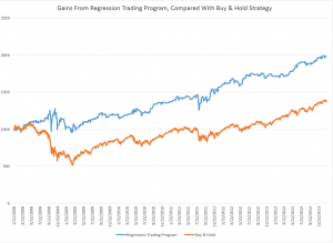
So here are the returns from applying this SPY from early 2008 to early 2014 (click to enlarge).

I begin with a $1000 investment 1/22/2008 and trade potentially every day, based on either the Trading Program or a Buy & Hold strategy.

Now there are several remarkable things about this Trading Program and the underlying regression model.

First, the regression model is a most unlikely candidate for making money in the stock market. The R²or coefficient of determination is 0.0238, implying that the 60 regressors predict only 2.38 percent of the variation in the SPY rates of return. And it’s possible to go on in this vein – for example, the F-statistic indicating whether there is a relation between the regressors and the dependent variable is 1.42, just marginally above the 1 percent significance level, according to my reading of the Tables.

And the regression with 60 regressors correctly predicts the correct sign of the next days’ SPY rates of return only 50.1 percent of the time.

This, of course, is a key fact, since the Trading Program (see below) is triggered by positive predictions of the next day’s rate of return. When the next day rate of return is predicted to be positive and above a certain minimum value, the Trading Program buys SPY with the money on hand from previous sales – or, if the investor is already holding SPY because the previous day’s prediction also was positive, the investor stands pat.

The Conventional Wisdom

Professor Jim Hamilton, one of the principals (with Menzie Chin) in Econbrowser had a post recently On R-squared and economic prediction which makes the sensible point that R² or the coefficient of determination in a regression is not a great guide to predictive performance. The post shows, among other things, that first differences of the daily S&P 500 index values regressed against lagged values of these first differences have low R² – almost zero.

Hamilton writes,

Actually, there’s a well-known theory of stock prices that claims that an R-squared near zero is exactly what you should find. Specifically, the claim is that everything anybody could have known last month should already have been reflected in the value of pt -1. If you knew last month, when pt-1 was 1800, that this month it was headed to 1900, you should have bought last month. But if enough savvy investors tried to do that, their buy orders would have driven pt-1 up closer to 1900. The stock price should respond the instant somebody gets the news, not wait around a month before changing.

That’s not a bad empirical description of stock prices– nobody can really predict them. If you want a little fancier model, modern finance theory is characterized by the more general view that the product of today’s stock return with some other characteristics of today’s economy (referred to as the “pricing kernel”) should have been impossible to predict based on anything you could have known last month. In this formulation, the theory is confirmed– our understanding of what’s going on is exactly correct– only if when regressing that product on anything known at t – 1 we always obtain an R-squared near zero.

Well, I’m in the position here of seeking to correct one of my intellectual mentors. Although Professor Hamilton and I have never met nor communicated directly, I did work my way through Hamilton’s seminal book on time series analysis – and was duly impressed.

I am coming to the opinion that the success of this fairly low-power regression model on the SPY must have to do with special characteristics of the underlying distribution of rates of return.

For example, it’s interesting that the correlations between the (61) regressors and the daily returns are higher, when the absolute values of the dependent variable rates of return are greater. There is, in fact, a lot of meaningless buzz at very low positive and negative rates of return. This seems consistent with the odd shape of the residuals of the regression, shown below.

I’ve made this point before, most recently in a post-2014 post Predicting the S&P 500 or the SPY Exchange-Traded Fund, where I actually provide coefficients for a autoregressive model estimated by Matlab’s arima procedure. That estimation, incidentally, takes more account of the non-normal characteristics of the distribution of the rates of return, employing a t-distribution in maximum likelihood estimates of the parameters. It also only uses lagged values of SPY daily returns, and does not include any contribution from the VIX.

I guess in the remote possibility Jim Hamilton glances at either of these posts, it might seem comparable to reading claims of a perpetual motion machine, a method to square the circle, or something similar- quackery or wrong-headedness and error.

A colleague with a Harvard Ph.D in applied math, incidentally, has taken the trouble to go over my data and numbers, checking and verifying I am computing what I say I am computing.

Further details follow on this simple ordinary least squares (OLS) regression model I am presenting here.

Data and the Model

The focus of this modeling effort is on the daily returns of the SPDR S&P 500 (SPY), calculated with daily closing prices, as -1+(today’s closing price/the previous trading day’s closing price). The data matrix includes 30 lagged values of the daily returns of the SPY (SPYRR) along with 30 lagged values of the daily returns of the VIX volatility index (VIXRR). The data span from 11/26/1993 to 1/16/2014 – a total of 5,072 daily returns.

There is enough data to create separate training and test samples, which is good, since in-sample performance can be a very poor guide to out-of-sample predictive capabilities. The training sample extends from 11/26/1993 to 1/18/2008, for a total of 3563 observations. The test sample is the complement of this, extending from 1/22/2008 to 1/16/2014, including 1509 cases.

So the basic equation I estimate is of the form

SPYRR_t=a₀+a₁SPYRR_t-1…a₃₀SPYRR_t-30+b₁VIXRR_t-1+..+b30VIXRR_t-30

Thus, the equation has 61 parameters – 60 coefficients multiplying into the lagged returns for the SPY and VIX indices and a constant term.

Estimation Technique

To make this simple, I estimate the above equation with the above data by ordinary least squares, implementing the standard matrix equation b = (X^TX)^-1X^TY, where T indicates ‘transpose.’ I add a leading column of ‘1’s’ to the data matrix X to allow for a constant term a₀. I do not mean center or standardize the observations on daily rates of return.

Rule for Trading Program and Summing UP

The Trading Program is the same one I described in earlier blog posts on this topic. Basically, I update forecasts every day and react to the forecast of the next day’s daily return. If it is positive, and now above a certain minimum, I either buy or hold. If it is not, I sell or do not enter the market. Oh yeah, I start out with $1000 in all these simulations and only trade with proceeds from this initial investment.

The only element of unrealism is that I have to predict the closing price of the SPY some short period before the close of the market to be able to enter my trade. I have not looked closely at this, but I am assuming volatility in the last few seconds is bounded, except perhaps in very unusual circumstances.

I take the trouble to present the results of an OLS regression to highlight the fact that what looks like a weak model in this context can work to achieve profits. I don’t think that point has ever been made. There are, of course, all sorts of possibilities for further optimizing this model.

I also suspect that monetary policy has some role in the success of this Trading Program over this period – so it would be interesting to look at similar models at other times and perhaps in other markets.

bagging, downloadable texts on statistics and forecasting, forecasting turning points, macroeconomic forecasting, random walk

The On-Coming Tsunami of Data Analytics

January 3, 2014 Clive Jones

More than 25,000 visited businessforecastblog, March 2012-December 2013, some spending hours on the site. Interest ran nearly 200 visitors a day in December, before my ability to post was blocked by a software glitch, and we did this re-boot.

Now I have hundreds of posts offline, pertaining to several themes, discussed below. How to put this material back up – as reposts, re-organized posts, or as longer topic summaries?

There’s a silver lining. This forces me to think through forecasting, predictive and data analytics.

One thing this blog does is compile information on which forecasting and data analytics techniques work, and, to some extent, how they work, how key results are calculated. I’m big on computation and performance metrics, and I want to utilize the SkyDrive more extensively to provide full access to spreadsheets with worked examples.

Often my perspective is that of a “line worker” developing sales forecasts. But there is another important focus – business process improvement. The strength of a forecast is measured, ultimately, by its accuracy. Efforts to improve business processes, on the other hand, are clocked by whether improvement occurs – whether costs of reaching customers are lower, participation rates higher, customer retention better or in stabilization mode (lower churn), and whether the executive suite and managers gain understanding of who the customers are. And there is a third focus – that of the underlying economics, particularly the dynamics of the institutions involved, such as the US Federal Reserve.

Right off, however, let me say there is a direct solution to forecasting sales next quarter or in the coming budget cycle. This is automatic forecasting software, with Forecast Pro being one of the leading products. Here’s a YouTube video with the basics about that product.

You can download demo versions and participate in Webinars, and attend the periodic conferences organized by Business Forecast Systems showcasing user applications in a wide variety of companies.

So that’s a good solution for starters, and there are similar products, such as the SAS/ETS time series software, and Autobox.

So what more would you want?

Well, there’s need for background information, and there’s a lot of terminology. It’s useful to know about exponential smoothing and random walks, as well as autoregressive and moving averages. Really, some reaches of this subject are arcane, but nothing is worse than a forecast setup which gains the confidence of stakeholders, and then falls flat on its face. So, yes, eventually, you need to know about “pathologies” of the classic linear regression (CLR) model – heteroscedasticity, autocorrelation, multicollinearity, and specification error!

And it’s good to gain this familiarity in small doses, in connection with real-world applications or even forecasting personalities or celebrities. After a college course or two, it’s easy to lose track of concepts. So you might look at this blog as a type of refresher sometimes.

Anticipating Turning Points in Time Series

But the real problem comes with anticipating turning points in business and economic time series. Except when modeling seasonal variation, exponential smoothing usually shoots over or under a turning point in any series it is modeling.

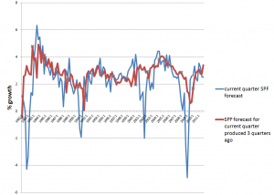
If this were easy to correct, macroeconomic forecasts would be much better. The following chart highlights the poor performance, however, of experts contributing to the quarterly Survey of Professional Forecasters, maintained by the Philadelphia Fed.

So, the red line is the SPF consensus forecast for GDP growth on a three quarter horizon, and the blue line is the forecast or nowcast for the current quarter (there is a delay in release of current numbers). Notice the huge dips in the current quarter estimate, associated with four recessions 1981, 1992, 2001-2, and 2008-9. A mere three months prior to these catastrophic drops in growth, leading forecasters at big banks, consulting companies, and universities totally missed the boat.

This is important in a practical sense, because recessions turn the world of many businesses upside down. All bets are off. The forecasting team is reassigned or let go as an economy measure, and so forth.

Some forward-looking information would help business intelligence focus on reallocating resources to sustain revenue as much as possible, using analytics to design cuts exerting the smallest impact on future ability to maintain and increase market share.

Hedgehogs and Foxes

Nate Silver has a great table in his best-selling The
Signal and the Noise on the qualities and forecasting performance of hedgehogs and foxes. The idea comes from a Greek poet, “The fox knows many little things, but the hedgehog knows one big thing.”

Following Tetlock, Silver finds foxes are multidisplinary, adaptable, self-critical, cautious, and empirical, tolerant of complexity. By contrast, the Hedgehog is specialized, sticks to the same approaches, stubbornly adheres to his model in spite of counter-evidence, is order-seeking, confident, and ideological. The evidence suggests foxes generally outperform hedgehogs, just as ensemble methods typically outperform a single technique in forecasting.

Message – be a fox.

So maybe this can explain some of the breadth of this blog. If we have trouble predicting GDP growth, what about forecasts in other areas – such as weather, climate change, or that old chestnut, sun spots? And maybe it is useful to take a look at how to forecast all the inputs and associated series – such as exchange rates, growth by global region, the housing market, interest rates, as well as profits.

And while we are looking around, how about brain waves? Can brain waves be forecast? Oh yes, it turns out there is a fascinating and currently applied new approach called neuromarketing, which uses headbands and electrodes, and even MRI machines, to detect deep responses of consumers to new products and advertising.

New Methods

I know I have not touched on cluster analysis and classification, areas making big contributions to improvement of business process. But maybe if we consider the range of “new” techniques for predictive analytics, we can see time series forecasting and analysis of customer behavior coming under one roof.

There is, for example, this many predictor thread emerging in forecasting in the late 1990’s and especially in the last decade with factor models for macroeconomic forecasting. Reading this literature, I’ve become aware of methods for mapping N explanatory variables onto a target variable, when there are M<N observations. These are sometimes called methods of data shrinkage, and include principal components regression, ridge regression, and the lasso. There are several others, and a good reference is The Elements of Statistical Learning, Data Mining, Learning and Prediction, 2nd edition, by Trevor Hastie, Robert Tibshirani, and Jerome Friedman. This excellent text is downloadable, accessible via the Tools, Apps, Texts, Free Stuff menu option located just to the left of the search utility on the heading for this blog.

There also is bagging, which is the topic of the previous post, as well as boosting, and a range of decision tree and regression tree modeling tactics, including random forests.

I’m actively exploring a number of these approaches, ginning up little examples to see how they work and how the computation goes. So far, it’s impressive. This stuff can really improve over the old approaches, which someone pointed out, have been around since the 1950’s at least.

It’s here I think that we can sight the on-coming wave, just out there on the horizon – perhaps hundreds of feet high. It’s going to swamp the old approaches, changing market research forever and opening new vistas, I think, for forecasting, as traditionally understood.

I hope to be able to ride that wave, and now I put it that way, I get a sense of urgency in keeping practicing my web surfing.

Hope you come back and participate in the comments section, or email me at [email protected]

bagging, forecasting turning points, random walk, Uncategorized

Changes to Businessforecastblog in 2014 – Where We Have Been, Where We Are Going

December 30, 2013 admin

We’ve been struggling with a software glitch in WordPress, due to, we think, incompatibilities between plug-in’s and a new version of the blogging software. It’s been pretty intense. The site has been fully up, but there was no possibility of new posts, not even a notice to readers about what was happening. All this started just before Christmas and ended, basically, yesterday.

So greetings. Count on daily posts as rule, and I will get some of the archives accessible ASAP.

But, for now, a few words about my evolving perspective.

I came out of the trenches, so to speak, of sales, revenue, and new product forecasting, for enterprise information technology (IT) and, earlier, for public utilities and state and federal agencies. When I launched Businessforecastblog last year, my bias popped up in the secondary heading for the blog – with its reference to “data-limited contexts” – and in early posts on topics like “simple trending” and random walks.

I essentially believed that most business and economic time series are basically one form or another of random walks, and that exponential smoothing is often the best forecasting approach in an applied context. Of course, this viewpoint can be bolstered by reference to research from the 1980’s by Nelson and Plosser and the M-Competitions. I also bought into a lazy consensus that it was necessary to have more observations than explanatory variables in order to estimate a multivariate regression. I viewed segmentation analysis, so popular in marketing research, as a sort of diversion from the real task of predicting responses of customers directly, based on their demographics, firmagraphics, and other factors.

So the press of writing frequent posts on business forecasting and related topics has led me to a learn a lot.

The next post to this blog, for example, will be about how “bagging” – from Bootstrap Aggregation – can radically reduce forecasting errors when there are only a few historical or other observations, but a large number of potential predictors. In a way, this provides a new solution to the problem of forecasting in data limited contexts.

This post also includes specific computations, in this case done in a spreadsheet. I’m big on actually computing stuff, where possible. I believe Elliot Shulman’s dictum, “you don’t really know something until you compute it.” And now I see how to include access to spreadsheets for readers, so there will be more of that.

Forecasting turning points is the great unsolved problem of business forecasting. That’s why I’m intensely interested in analysis of what many agree are asset bubbles. Bursting of the dot.com bubble initiated the US recession of 2001. Collapse of the housing market and exotic financial instrument bubbles in 2007 bought on the worst recession since World War II, now called the Great Recession. If it were possible to forecast the peak of various asset bubbles, like researchers such as Didier Sornette suggest, this would mean we would have some advance – perhaps only weeks of course – on the onset of the next major business turndown.

Along the way, there are all sorts of interesting sidelights relating to business forecasting and more generally predictive analytics. In fact, it’s clear that in the era of Big Data, data analytics can contribute to improvement of business processes – things like target marketing for customers – as well as perform less glitzy tasks of projecting sales for budget formulation and the like.

Email me at [email protected] if you want to receive PDF compilations on topics from the archives. I’m putting together compilations on New Methods and Asset Bubbles, for starters, in a week or so.

Business Forecasting