March 25, 2009, Goldman Sachs’ Commodity and Strategy Research group published Global Economics Paper No 183: Forecasting Gold as a Commodity.

This offers a fascinating overview of supply and demand in global gold markets and an immediate prediction –

This “gold as a commodity” framework suggests that gold prices have strong support at and above current price levels should the current low real interest rate environment persist. Specifically, assuming real interest rates stay near current levels and the buying from gold-ETFs slows to last year’s pace, we would expect to see gold prices stay near $930/toz over the next six months, rising to $962/toz on a 12-month horizon.

The World Gold Council maintains an interactive graph of gold prices based on the London PM fix.

Now, of course, the real interest rate is an inflation-adjusted nominal interest rate. It’s usually estimated as a difference between some representative interest rate and relevant rate of inflation. Thus, the real interest rates in the Goldman Sachs report is really an extrapolation from extant data provided, for example, by the US Federal Reserve FRED database.

Gratis of Paul Krugman’s New York Times blog from last August, we have this time series for real interest rates –

The graph shows that “real interest rates stay near current levels” (from spring 2009), putting the Goldman Sachs group authoring Report No 183 on record as producing one of the most successful longer term forecasts that you can find.

I’ve been collecting materials on forecasting systems for gold prices, and hope to visit that topic in coming posts here.

climate change, long term forecasting, present value accounting

Forecasting – Climate Change and Infrastructure

March 12, 2014 Clive Jones

You really have to become something like a social philosopher to enter the climate change and infrastructure discussion. I mean this several ways.

Of course, there is first the continuing issue of whether or not climate change is real, or is currently being reversed by a “pause” due to the oceans or changes in trade winds absorbing some of the increase in temperatures. So for purposes of discussion, I’m going to assume that climate change is real, and with a new El Niño this year global temperatures and a whole panoply of related weather phenomena – like major hurricanes – will come back in spades.

But then can we do anything about it? Is it possible for a developed or “mature” society to plan for an uncertain, but increasingly likely future? With this question come visions of the amazingly dysfunctional US Congress, mordantly satirized in the US TV show House of Cards.

The National Society of Professional Engineers points out that major infrastructure bills relating to funding the US highway system and water systems are coming up in Congress in 2014.

Desperately needed long-term infrastructure projects were deferred to address other national priorities or simply fell victim to the ongoing budget crisis. In fact, federal lawmakers extended the surface transportation authorization an unprecedented 10 times between 2005 and 2012, when Congress finally authorized the two-year Moving Ahead for Progress in the 21^st Century Act (MAP-21). Now, with MAP-21 set to expire before the end of 2014, two of the most significant pieces of infrastructure legislation are taking center stage in Congress. The Water Resources Reform and Development Act (WRRDA) and the reauthorization of the surface transportation bill present a rare opportunity for Congress to set long-term priorities and provide needed investment in our nation’s infrastructure. Collectively, these two bills cover much, though not all, of US infrastructure. The question then becomes, can Congress overcome continuing partisan gridlock and a decades-long pattern of short-term fixes to make a meaningful commitment to the long-term needs of US infrastructure?

Yes, for sure, that is the question.

Hurricane Sandy – really by the time it hit New Jersey and New York a fierce tropical storm – wreaked havoc on Far Rockaway, flooding the New York City subway system in 2012. This gave rise to talk of sea walls after the event. And I assume something like that is in the planning stages on drawing boards somewhere on the East Coast. But the cost of “ten story tall pilings” on which would be hinged giant gates is on the order of billions of US dollars.

California

I notice interesting writing coming out of California, pertaining to the smart grid and the need to extend this concept from electricity to water.

The California Energy Commission (CEC) publishes an Integrated Energy Policy Report (IEPR – pronounced eye-per) every two years, and the 2013 IEPR was just approved ..Let’s look at two climate change impacts – temperature and precipitation. From a temperature perspective, the IEPR anticipates that as the thermometer rises, so does the demand for electricity to run AC. San Francisco Peninsula communities that never had a need for AC will install a couple million units to deal with summer temperatures formerly confined to the Central Valley. PG&E and municipal utilities in Northern California will notice impacts in seasonal demand for electricity in both the duration of heat waves and peak apexes during the hottest times of day. In the southern part of the state, the demand will also grow as AC units work harder to offset hotter days. At the same time, increased temperatures decrease power plant efficiencies, whether the plant generates electricity from natural gas, solar thermal, nuclear, or geothermal. Their cooling processes are also negatively impacted by heat waves. Increased temperatures also impact transmission lines – reducing their efficiency and creating line sags that can trigger service disruptions. Then there’s precipitation. Governor Jerry Brown just announced a drought emergency for the state. A significant portion of California’s water storage system relies on the Sierra Mountains snowpack, which is frighteningly low this winter. This snowpack supplies most of the water sourced within the state, and hydropower derived from it supplies about 15% of the state’s homegrown electricity. A hotter climate means snowfall becomes rainfall, and it is no longer freely stored as snow that obligingly melts as temperatures rise. It may not be as reliably scheduled for generation of hydro power as snowfalls shift to rainfalls. We may also receive less precipitation as a result of climate change – that’s a big unknown right now. One thing is certain. A hotter climate will require more water for agriculture – a $45 billion economy in California – to sustain crops. And whether it is water for industrial, commercial, agricultural, or residential uses, what doesn’t fall from the skies will require electricity to pump it, transport it, desalinate it, or treat it.

Boom – A Journal of California packs more punch in discussing the “worst case”

“The choice before us is not to stop climate change,” says Jonathan Parfrey, executive director of Climate Resolve in Los Angeles. “That ship has sailed. There’s no going back. There will be impacts. The choice that’s before humanity is how bad are we going to do it to ourselves?”

So what will it be? Do you want the good news or the bad news first?

The bad news. OK.

If we choose to do nothing, the nightmare scenario plays out something like this: amid prolonged drought conditions, wildfires continuously burn across a dust-dry landscape, while potable water has become such a precious commodity that watering plants is a luxury only residents of elite, gated communities can afford. Decimated by fires, the power grid infrastructure that once distributed electricity—towers and wires—now loom as ghostly relics stripped of function. Along the coast, sea level rise has decimated beachfront properties while flooding from frequent superstorms has transformed underground systems, such as Bay Area Rapid Transit (BART), into an unintended, unmanaged sewer system..

This article goes on to the “good news” which projects a wave of innovations and green technology by 2050 to 2075 in California.

Sea Level Rise

Noone knows, at this point, the extent of the rise in sea level in coming years, and interestingly, I never seen a climate change denier also, in the same breath, deny that sea levels have been rising historically.

There are interesting resources on sea level rise, although projections of how much rise over what period are uncertain, because no one knows whether a big ice mass, such as parts of the Antarctic ice shelf are going to melt on an accelerated schedule sometime soon.

An excellent scientific summary of the sea level situation historically can be found in Understanding global sea levels: past, present and future.

Here is an overall graph of Global Mean Sea Level –

This inexorable trend has given rise to map resources which suggest coastal areas which would be underwater or adversely affected in the future by sea surges.

The New York Times’ interactive What Could Disappear suggests Boston might look like this, with a five foot rise in sea level expected by 2100

The problem, of course, is that globally populations are concentrated in coastal areas.

Also, storm surges are nonlinearly related to sea level. Thus, a one (1) foot rise in sea level could be linked with significantly more than 1 foot increases in the height of storm surges.

Longer Term Forecasts

Some years back, an interesting controversy arose over present value discounting in calculating impacts of climate change.

So, currently, the medium term forecasts of climate change impacts – sea level rises of maybe 1 to 2 feet, average temperature increases of one or two degrees, and so forth – seem roughly manageable. The problem always seems to come in the longer term – after 2100 for example in the recent National Academy of Sciences study funded, among others, by the US intelligence community.

The problem with calculating the impacts and significance of these longer term impacts today is that the present value accounting framework just makes things that far into the future almost insignificant.

Currently, for example, global output is on the order of 80 trillion dollars. Suppose we accept a discount rate of 4 percent. Then, calculating the discount factor 150 years from today, in 2154, we have 0 .003. So according to this logic, the loss of 80 trillion dollars worth of production in 2154 has a present value of about 250 billion dollars. Thus, losing an amount of output in 150 years equal to the total productive activity of the planet today is worth a mere 250 billion dollars in present value terms, or about the current GDP of Ireland.

Now I may have rounded and glossed some of the arithmetic possibly, but the point stands no matter how you make the computation.

This is totally absurd. Because as a guide to losing future output of $80 trillion dollars in a century and one half, it seems we should be willing to spend on a planetary basis more than a one-time cost of $35 per person today, when the per capita global output is on the order of $1000 per person.

So we need a better accounting framework.

Of course, there are counterarguments. For example, in 150 years, perhaps science will have discovered how to boost the carbon dioxide processing capabilities of plants, so we can have more pollution. And looking back 150 years to the era of the horse and buggy, we can see that there has been tremendous technological change.

But this is a little like waiting for the amazing “secret weapons” to be unveiled in a war you are losing.

Header photo courtesy of NASA

geopolitical risk, global business forecasts

Geopolitical Outlook 2014

March 11, 2014 Clive Jones

One service forecasting “staff” can provide executives and managers is a sort of list of global geopolitical risks. This is compelling only at certain times – and 2014 and maybe 2015 seem to be shaping up as one of these periods.

Just a theory, but, in my opinion, the sustained lackluster economic performance in the global economy, especially in Europe and also, by historic standards, the United States adds fuel to the fire of many conflicts. Conflict intensifies as people fight over an economic pie that is shrinking, or at least, not getting appreciably bigger, despite population growth and the arrival of new generations of young people on the scene.

Some Hotspots

Asia

First, the recent election in Thailand solved nothing, so far. The tally of results looks like it is going to take months – sustaining a kind of political vacuum after many violent protests. Economic growth is impacted, and the situation looks to be fluid.

But the big issue is whether China is going to experience significantly slower economic growth in 2014-2015, and perhaps some type of debt crisis.

For the first time, we are seeing municipal bond defaults and the run-on effects are not pretty.

The default on a bond payment by China’s Chaori Solar last week signalled a reassessment of credit risk in a market where even high-yielding debt had been seen as carrying an implicit state guarantee. On Tuesday, another solar company announced a second year of net losses, leading to a suspension of its stock and bonds on the Shanghai stock exchange and stoking fears that it, too, may default.

There are internal and external forces at work in the Chinese situation. It’s important to remember lackluster growth in Europe, one of China’s biggest customers, is bound to exert continuing downward pressure on Chinese economic growth.

Michael Pettis addresses some of these issues in his recent post Will emerging markets come back? Concluding that –

Emerging markets may well rebound strongly in the coming months, but any rebound will face the same ugly arithmetic. Ordinary households in too many countries have seen their share of total GDP plunge. Until it rebounds, the global imbalances will only remain in place, and without a global New Deal, the only alternative to weak demand will be soaring debt. Add to this continued political uncertainty, not just in the developing world but also in peripheral Europe, and it is clear that we should expect developing country woes only to get worse over the next two to three years.

Indonesia is experiencing persisting issues with the stability of its currency.

Europe

In general, economic growth in Europe is very slow, tapering to static and negative growth in key economies and the geographic periphery.

The European Commission, the executive arm of the European Union, on Tuesday forecast growth in the 28-county EU at 1.5 per cent this year and 2 per cent in 2015. But growth in the 18 euro zone countries, many of which are weighed down by high debt and lingering austerity, is forecast at only 1.2 per cent this year, up marginally from 1.1 per cent in the previous forecast, and 1.8 per cent next year.

France avoided recession by posting 0.3 % GDP in the final quarter of calendar year 2013.

Since margin of error for real GDP forecasts is on the order of +/- 2 percent, current forecasts are, in many cases, indistinguishable from a prediction of another recession.

And what could cause such a wobble?

Well, possibly increases in natural gas prices, as a result of political conflict between Russia and the west, or perhaps the outbreak of civil war in various eastern European locales?

The Ukraine

The issue of the Ukraine is intensely ideological and politicized and hard to evaluate without devolving into propaganda.

The population of the Ukraine has been in radical decline. Between 1991 and 2011 the Ukrainian population decreased by 11.8%, from 51.6 million to 45.5 million, apparently the result of very low fertility rates and high death rates. Transparency International also rates the Ukraine 144^th out of 177^th in terms of corruption – with 177^th being worst.

“Market reforms” such as would come with an International Monetary Fund (IMF) loan package would probably cause further hardship in the industrialized eastern areas of the country.

Stratfor and other emphasize the role of certain “oligarchs” in the Ukraine, operating more or less behind the scenes. I take it these immensely rich individuals in many cases were the beneficiaries of privatization of former state enterprise assets.

The Middle East

Again, politics is supreme. Political alliances between Saudi Arabia and others seeking to overturn Assad in Syria create special conditions, for sure. The successive governments in Egypt, apparently returning to rule by a strongman, are one layer – another layer is the increasingly challenged economic condition in the country – where fuel subsidies are commonly doled out to many citizens. Israel, of course, is a focus of action and reaction, and under Netanyahu is more than ready to rattle the sword. After Iraq and Afghanistan, it seems always possible for conflict to break out in unexpected directions in this region of the world.

A situation seems to be evolving in Turkey, which I do not understand, but may be involved with corruption scandals and spillovers from conflicts not only Syria but also the Crimea.

The United States

A good part of the US TV viewing audience has watched part or all of House of Cards, the dark, intricate story of corruption and intrigue at the highest levels of the US Congress. This show reinforces the view, already widely prevalent, that US politicians are just interested in fund-raising and feathering their own nest, and that they operate more or less in callous disregard or clear antagonism to the welfare of the people at large.

This is really too bad, in a way, since more than ever the US needs people to participate in the political process.

I wonder whether the consequence of this general loss of faith in the powers that be might fall naturally into the laps of more libertarian forces in US politics. State control and policies are so odious – how about trimming back the size of the central government significantly, including its ability to engage in foreign military and espionage escapades? Shades of Ron Paul and maybe his son, Senator Rand Paul of Kentucky.

South and Central America

Brazil snagged the Summer 2016 Olympics and is rushing to construct an ambitious number of venues around that vast country.

While the United States was absorbed in wars in the Middle East, an indigenous, socialist movement emerged in South American – centered around Venezuela and perhaps Bolivia, or Chile and Argentina. At least in Venezuela, sustaining these left governments after the charismatic leader passes from the scene is proving difficult.

Africa

Observing the ground rule that this sort of inventory has to be fairly easy, in order to be convincing – it seems that conflict is the order of the day across Africa. At the same time, the continent is moving forward, experiencing economic development, dealing with AIDS. Perhaps the currency situation in South Africa is the biggest geopolitical risk.

Bottom Line

The most optimistic take is that the outlook and risks now define a sort of interim period, perhaps lasting several years, when the level of conflict will increase at various hotspots. The endpoint, hopefully, will be the emergence of new technologies and products, new industries, which will absorb everyone in more constructive growth – perhaps growth defined ecologically, rather than merely in counting objects.

accuracy of forecasts, Big Data, data reduction, data science, financial forecasting, financial forecasts, macroeconomic forecasting, many predictors, partial least squares, predictive analytics, three pass regression filter (3PRF)

Three Pass Regression Filter – New Data Reduction Method

March 10, 2014 Clive Jones

Malcolm Gladwell’s 10,000 hour rule (for cognitive mastery) is sort of an inspiration for me. I picked forecasting as my field for “cognitive mastery,” as dubious as that might be. When I am directly engaged in an assignment, at some point or other, I feel the need for immersion in the data and in estimations of all types. This blog, on the other hand, represents an effort to survey and, to some extent, get control of new “tools” – at least in a first pass. Then, when I have problems at hand, I can try some of these new techniques.

Ok, so these remarks preface what you might call the humility of my approach to new methods currently being innovated. I am not putting myself on a level with the innovators, for example. At the same time, it’s important to retain perspective and not drop a critical stance.

The Working Paper and Article in the Journal of Finance

Probably one of the most widely-cited recent working papers is Kelly and Pruitt’s three pass regression filter (3PRF). The authors, shown above, are with the University of Chicago, Booth School of Business and the Federal Reserve Board of Governors, respectively, and judging from the extensive revisions to the 2011 version, they had a bit of trouble getting this one out of the skunk works.

Recently, however, Kelly and Pruit published an important article in the prestigious Journal of Finance called Market Expectations in the Cross-Section of Present Values. This article applies a version of the three pass regression filter to show that returns and cash flow growth for the aggregate U.S. stock market are highly and robustly predictable.

I learned of a published application of the 3PRF from Francis X. Dieblod’s blog, No Hesitations, where Diebold – one of the most published authorities on forecasting – writes

Recent interesting work, moreover, extends PLS in powerful ways, as with the Kelly-Pruitt three-pass regression filter and its amazing apparent success in predicting aggregate equity returns.

What is the 3PRF?

The working paper from the Booth School of Business cited at a couple of points above describes what might be cast as a generalization of partial least squares (PLS). Certainly, the focus in the 3PRF and PLS is on using latent variables to predict some target.

I’m not sure, though, whether 3PRF is, in fact, more of a heuristic, rather than an algorithm.

What I mean is that the three pass regression filter involves a procedure, described below.

(click to enlarge).

Here’s the basic idea –

Suppose you have a large number of potential regressors x_i ε X, i=1,..,N. In fact, it may be impossible to calculate an OLS regression, since N > T the number of observations or time periods.

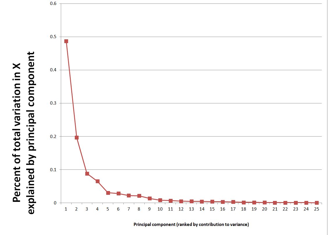
Furthermore, you have proxies z_j ε Z, I = 1,..,L – where L is significantly less than the number of observations T. These proxies could be the first several principal components of the data matrix, or underlying drivers which theory proposes for the situation. The authors even suggest an automatic procedure for generating proxies in the paper.

And, finally, there is the target variable y_t which is a column vector with T observations.

Latent factors in a matrix F drive both the proxies in Z and the predictors in X. Based on macroeconomic research into dynamic factors, there might be only a few of these latent factors – just as typically only a few principal components account for the bulk of variation in a data matrix.

Now here is a key point – as Kelly and Pruitt present the 3PRF, it is a leading indicator approach when applied to forecasting macroeconomic variables such as GDP, inflation, or the like. Thus, the time index for y_t ranges from 2,3,…T+1, while the time indices of all X and Z variables and the factors range from 1,2,..T. This means really that all the x and z variables are potentially leading indicators, since they map conditions from an earlier time onto values of a target variable at a subsequent time.

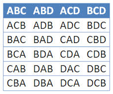
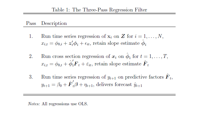
What Table 1 above tells us to do is –

Run an ordinary least square (OLS) regression of the x_i in X onto the z_j in X, where T ranges from 1 to T and there are N variables in X and L << T variables in Z. So, in the example discussed below, we concoct a spreadsheet example with 3 variables in Z, or three proxies, and 10 predictor variables x_i in X (I could have used 50, but I wanted to see whether the method worked with lower dimensionality). The example assumes 40 periods, so t = 1,…,40. There will be 40 different sets of coefficients of the z_j as a result of estimating these regressions with 40 matched constant terms.
OK, then we take this stack of estimates of coefficients of the z_j and their associated constants and map them onto the cross sectional slices of X for t = 1,..,T. This means that, at each period t, the values of the cross-section. x_i,t, are taken as the dependent variable, and the independent variables are the 40 sets of coefficients (plus constant) estimated in the previous step for period t become the predictors.
Finally, we extract the estimate of the factor loadings which results, and use these in a regression with target variable as the dependent variable.

This is tricky, and I have questions about the symbolism in Kelly and Pruitt’s papers, but the procedure they describe does work. There is some Matlab code here alongside the reference to this paper in Professor Kelly’s research.

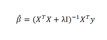
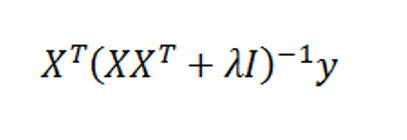
At the same time, all this can be short-circuited (if you have adequate data without a lot of missing values, apparently) by a single humungous formula –

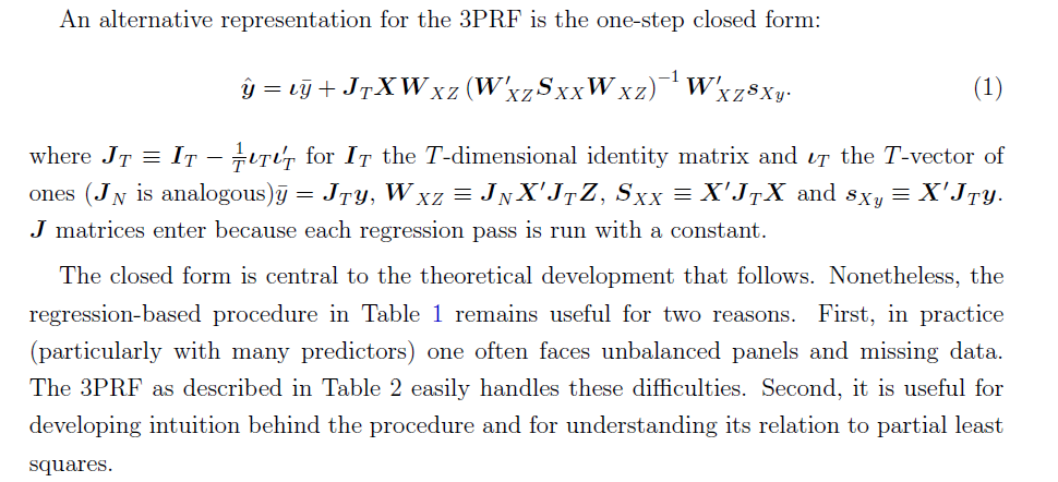
Here, the source is the 2012 paper.

Spreadsheet Implementation

Spreadsheets help me understand the structure of the underlying data and the order of calculation, even if, for the most part, I work with toy examples.

So recently, I’ve been working through the 3PRF with a small spreadsheet.

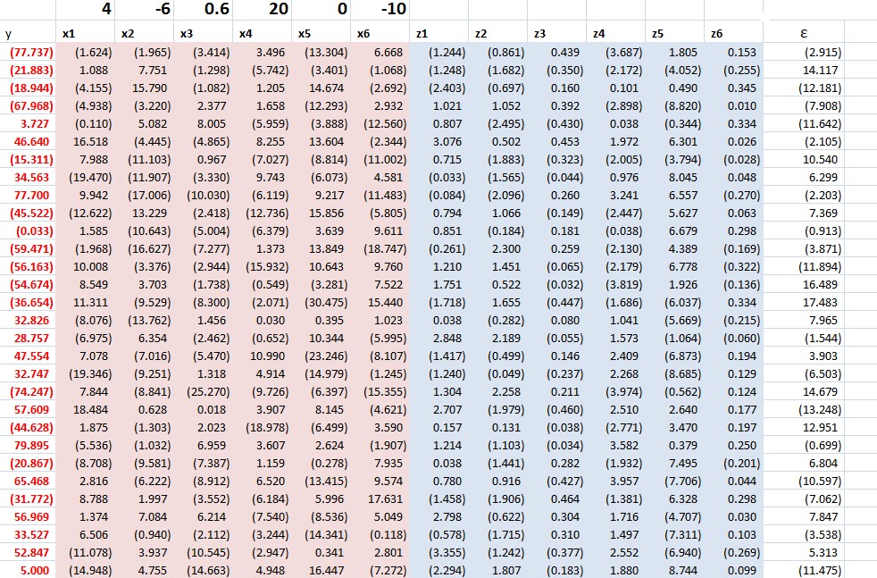
Generating the factors:I generated the factors as two columns of random variables (=rand()) in Excel. I gave the factors different magnitudes by multiplying by different constants.

Generating the proxies Z and predictors X. Kelly and Pruitt call for the predictors to be variance standardized, so I generated 40 observations on ten sets of x_iby selecting ten different coefficients to multiply into the two factors, and in each case I added a normal error term with mean zero and standard deviation 1. In Excel, this is the formula =norminv(rand(),0,1).

Basically, I did the same drill for the three z_j — I created 40 observations for z1, z2, and z3 by multiplying three different sets of coefficients into the two factors and added a normal error term with zero mean and variance equal to 1.

Then, finally, I created y_t by multiplying randomly selected coefficients times the factors.

After generating the data, the first pass regression is easy. You just develop a regression with each predictor x_i as the dependent variable and the three proxies as the independent variables, case-by-case, across the time series for each. This gives you a bunch of regression coefficients which, in turn, become the explanatory variables in the cross-sectional regressions of the second step.

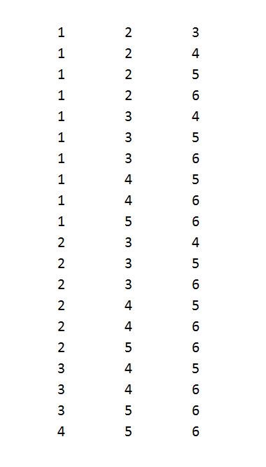
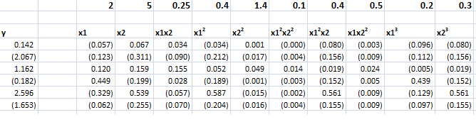
The regression coefficients I calculated for the three proxies, including a constant term, were as follows – where the 1^st row indicates the regression for x₁ and so forth.

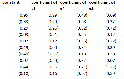
This second step is a little tricky, but you just take all the values of the predictor variables for a particular period and designate these as the dependent variables, with the constant and coefficients estimated in the previous step as the independent variables. Note, the number of predictors pairs up exactly with the number of rows in the above coefficient matrix.

This then gives you the factor loadings for the third step, where you can actually predict y_t (really y_t+1 in the 3PRF setup). The only wrinkle is you don’t use the constant terms estimated in the second step, on the grounds that these reflect “idiosyncratic” effects, according to the 2011 revision of the paper.

Note the authors describe this as a time series approach, but do not indicate how to get around some of the classic pitfalls of regression in a time series context. Obviously, first differencing might be necessary for nonstationary time series like GDP, and other data massaging might be in order.

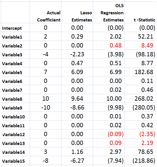
Bottom line – this worked well in my first implementation.

To forecast, I just used the last regression for y_t+1 and then added ten more cases, calculating new values for the target variable with the new values of the factors. I used the new values of the predictors to update the second step estimate of factor loadings, and applied the last third pass regression to these values.

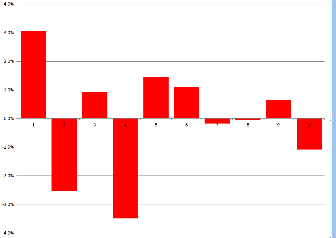
Here are the forecast errors for these ten out-of-sample cases.

Not bad for a first implementation.

Why Is Three Pass Regression Important?

3PRF is a fairly “clean” solution to an important problem, relating to the issue of “many predictors” in macroeconomics and other business research.

Noting that if the predictors number near or more than the number of observations, the standard ordinary least squares (OLS) forecaster is known to be poorly behaved or nonexistent, the authors write,

How, then, does one effectively use vast predictive information? A solution well known in the economics literature views the data as generated from a model in which latent factors drive the systematic variation of both the forecast target, y, and the matrix of predictors, X. In this setting, the best prediction of y is infeasible since the factors are unobserved. As a result, a factor estimation step is required. The literature’s benchmark method extracts factors that are significant drivers of variation in X and then uses these to forecast y. Our procedure springs from the idea that the factors that are relevant to y may be a strict subset of all the factors driving X. Our method, called the three-pass regression filter (3PRF), selectively identifies only the subset of factors that influence the forecast target while discarding factors that are irrelevant for the target but that may be pervasive among predictors. The 3PRF has the advantage of being expressed in closed form and virtually instantaneous to compute.

So, there are several advantages, such as (1) the solution can be expressed in closed form (in fact as one complicated but easily computable matrix expression), and (2) there is no need to employ maximum likelihood estimation.

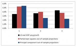
Furthermore, 3PRF may outperform other approaches, such as principal components regression or partial least squares.

The paper illustrates the forecasting performance of 3PRF with real-world examples (as well as simulations). The first relates to forecasts of macroeconomic variables using data such as from the Mark Watson database mentioned previously in this blog. The second application relates to predicting asset prices, based on a factor model that ties individual assets’ price-dividend ratios to aggregate stock market fluctuations in order to uncover investors’ discount rates and dividend growth expectations.

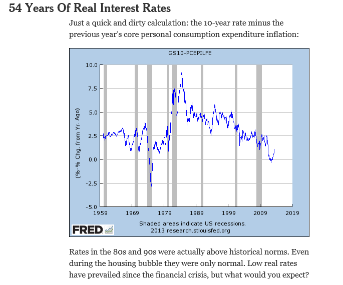
accuracy of forecasts, Big Data, data science, downloadable texts on statistics and forecasting, macroeconomic forecasting, many predictors, partial least squares, predictive analytics, principal component models and forecasts

Partial Least Squares and Principal Components

March 9, 2014 Clive Jones

I’ve run across outstanding summaries of “partial least squares” (PLS) research recently – for example Rosipal and Kramer’s Overview and Recent Advances in Partial Least Squares and the 2010 Handbook of Partial Least Squares.

Partial least squares (PLS) evolved somewhat independently from related statistical techniques, owing to what you might call family connections. The technique was first developed by Swedish statistician Herman Wold and his son, Svante Wold, who applied the method in particular to chemometrics. Rosipal and Kramer suggest that the success of PLS in chemometrics resulted in a lot of applications in other scientific areas including bioinformatics, food research, medicine, [and] pharmacology..

Someday, I want to look into “path modeling” with PLS, but for now, let’s focus on the comparison between PLS regression and principal component (PC) regression. This post develops a comparison with Matlab code and macroeconomics data from Mark Watson’s website at Princeton.

The Basic Idea Behind PC and PLS Regression

Principal component and partial least squares regression share a couple of features.

Both, for example, offer an approach or solution to the problem of “many predictors” and multicollinearity. Also, with both methods, computation is not transparent, in contrast to ordinary least squares (OLS). Both PC and PLS regression are based on iterative or looping algorithms to extract either the principal components or underlying PLS factors and factor loadings.

PC Regression

The first step in PC regression is to calculate the principal components of the data matrix X. This is a set of orthogonal (which is to say completely uncorrelated) vectors which are weighted sums of the predictor variables in X.

This is an iterative process involving transformation of the variance-covariance or correlation matrix to extract the eigenvalues and eigenvectors.

Then, the data matrix X is multiplied by the eigenvectors to obtain the new basis for the data – an orthogonal basis. Typically, the first few (the largest) eigenvalues – which explain the largest proportion of variance in X – and their associated eigenvectors are used to produce one or more principal components which are regressed onto Y. This involves a dimensionality reduction, as well as elimination of potential problems of multicollinearity.

PLS Regression

The basic idea behind PLS regression, on the other hand, is to identify latent factors which explain the variation in both Y and X, then use these factors, which typically are substantially fewer in number than k, to predict Y values.

Clearly, just as in PC regression, the acid test of the model is how it performs on out-of-sample data.

The reason why PLS regression often outperforms PC regression, thus, is that factors which explain the most variation in the data matrix may not, at the same time, explain the most variation in Y. It’s as simple as that.

Matlab example

I grabbed some data from Mark Watson’s website at Princeton — from the links to a recent paper called Generalized Shrinkage Methods for Forecasting Using Many Predictors (with James H. Stock), Journal of Business and Economic Statistics, 30:4 (2012), 481-493.Download Paper (.pdf). Download Supplement (.pdf), Download Data and Replication Files (.zip). The data include the following variables, all expressed as year-over-year (yoy) growth rates: The first variable – real GDP – is taken as the forecasting target. The time periods of all other variables are lagged one period (1 quarter) behind the quarterly values of this target variable.

Matlab makes calculation of both principal component and partial least squares regressions easy.

The command to extract principal components is

[coeff, score, latent]=princomp(X)

Here X the data matrix, and the entities in the square brackets are vectors or matrices produced by the algorithm. It’s possible to compute a principal components regression with the contents of the matrix score. Generally, the first several principal components are selected for the regression, based on the importance of a component or its associated eigenvalue in latent. The following scree chart illustrates the contribution of the first few principal components to explaining the variance in X.

The relevant command for regression in Matlab is

b=regress(Y,score(:,1:6))

where b is the column vector of estimated coefficients and the first six principal components are used in place of the X predictor variables.

The Matlab command for a partial least square regresssion is

[XL,YL,XS,YS,beta] = plsregress(X,Y,ncomp)

where ncomp is the number of latent variables of components to be utilized in the regression. There are issues of interpreting the matrices and vectors in the square brackets, but I used this code –

data=xlsread(‘stock.xls’); X=data(1:47,2:79); y = data(2:48,1);

[XL,yl,XS,YS,beta] = plsregress(X,y,10); yfit = [ones(size(X,1),1) X]*beta;

lookPLS=[y yfit]; ZZ=data(48:50,2:79);newy=data(49:51,1);

new=[ones(3,1) ZZ]*beta; out=[newy new];

The bottom line is to test the estimates of the response coefficients on out-of-sample data.

The following chart shows that PLS outperforms PC, although the predictions of both are not spectacularly accurate.

Commentary

There are nuances to what I have done which help explain the dominance of PLS in this situation, as well as the weakly predictive capabilities of both approaches.

First, the target variable is quarterly year-over-year growth of real US GDP. The predictor set X contains 78 other macroeconomic variables, all expressed in terms of yoy (year-over-year) percent changes.

Again, note that the time period of all the variables or observations in X are lagged one quarter from the values in Y, or the values or yoy quarterly percent growth of real US GDP.

This means that we are looking for a real, live leading indicator. Furthermore, there are plausibly common factors in the Y series shared with at least some of the X variables. For example, the percent changes of a block of variables contained in real GDP are included in X, and by inspection move very similarly with the target variable.

Other Example Applications

There are at least a couple of interesting applied papers in the Handbook of Partial Least Squares – a downloadable book in the Springer Handbooks of Computational Statistics. See –

Chapter 20 A PLS Model to Study Brand Preference: An Application to the Mobile Phone Market

Chapter 22 Modeling the Impact of Corporate Reputation on Customer Satisfaction and Loyalty Using Partial Least Squares

Another macroeconomics application from the New York Fed –

“Revisiting Useful Approaches to Data-Rich Macroeconomic Forecasting”

http://www.newyorkfed.org/research/staff_reports/sr327.pdf

Finally, the software company XLStat has a nice, short video on partial least squares regression applied to a marketing example.

Big Data, data science

Links – March 7, 2014

March 8, 2014 Clive Jones

Stuff is bursting out all over, more or less in anticipation of the spring season – or World War III, however you might like to look at it. So I offer an assortment of links to topics which are central and interesting below.

Human Longevity Inc. (HLI) Launched to Promote Healthy Aging Using Advances in Genomics and Stem Cell Therapies Craig Venter – who launched a competing private and successful effort to map the human genome – is involved with this. Could be important.

MAA Celebrates Women’s History Month In celebration of Women’s History Month, the MAA has collected photographs and brief bios of notable female mathematicians from its Women of Mathematics poster. Emma Noether shown below – “mother” of Noetherian rings and other wonderous mathematical objects.

Three Business Benefits of Cloud Computing – price, access, and security

Welcome to the Big Data Economy This is the first chapter of a new eBook that details the 4 ways the future of data is cleaner, leaner, and smarter than its storied past. Download the entire eBook, Big Data Economy, for free here

Financial Sector Ignores Ukraine, Pushing Stocks Higher From March 6, video on how the Ukraine crisis has been absorbed by the market.

Employment-Population ratio Can the Fed reverse this trend?

How to Predict the Next Revolution

…few people noticed an April 2013 blog post by British academic Richard Heeks, who is director of the University of Manchester’s Center for Development Informatics. In that post, Heeks predicted the Ukrainian revolution.

A e-government expert, Heeks devised his “Revolution 2.0” index as a toy or a learning tool. The index combines three elements: Freedom House’s Freedom on the Net scores, the International Telecommunication Union’s information and communication technology development index, and the Economist’s Democracy Index (reversed into an “Outrage Index” so that higher scores mean more plutocracy). The first component measures the degree of Internet freedom in a country, the second shows how widely Internet technology is used, and the third supplies the level of oppression.

“There are significant national differences in both the drivers to mass political protest and the ability of such protest movements to freely organize themselves online,” Heeks wrote. “Both of these combine to give us some sense of how likely ‘mass protest movements of the internet age’ are to form in any given country.”

Simply put, that means countries with little real-world democracy and a lot of online freedom stand the biggest chance of a Revolution 2.0. In April 2013, Ukraine topped Heeks’s list, closely followed by Argentina and Georgia. The Philippines, Brazil, Russia, Kenya, Nigeria, Azerbaijan and Jordan filled out the top 10.

Proletarian Robots Getting Cheaper to Exploit Good report on a Russian robot conference recently.

The Top Venture Capital Investors By Exit Activity – Which Firms See the Highest Share of IPOs?

bagging, Big Data, complete subset regression, data science, financial forecasts, variable selection

Complete Subset Regressions

March 5, 2014 Clive Jones

A couple of years or so ago, I analyzed a software customer satisfaction survey, focusing on larger corporate users. I had firmagraphics – specifying customer features (size, market segment) – and customer evaluation of product features and support, as well as technical training. Altogether, there were 200 questions that translated into metrics or variables, along with measures of customer satisfaction. Altogether, the survey elicited responses from about 5000 companies.

Now this is really sort of an Ur-problem for me. How do you discover relationships in this sort of data space? How do you pick out the most important variables?

Since researching this blog, I’ve learned a lot about this problem. And one of the more fascinating approaches is the recent development named complete subset regressions.

And before describing some Monte Carlo exploring this approach here, I’m pleased Elliot, Gargano, and Timmerman (EGT) validate an intuition I had with this “Ur-problem.” In the survey I mentioned above, I calculated a whole bunch of univariate regressions with customer satisfaction as the dependent variable and each questionnaire variable as the explanatory variable – sort of one step beyond calculating simple correlations. Then, it occurred to me that I might combine all these 200 simple regressions into a predictive relationship. To my surprise, EGT’s research indicates that might have worked, but not be as effective as complete subset regression.

Complete Subset Regression (CSR) Procedure

As I understand it, the idea behind CSR is you run regressions with all possible combinations of some number r less than the total number n of candidate or possible predictors. The final prediction is developed as a simple average of the forecasts from these regressions with r predictors. While some of these regressions may exhibit bias due to specification error and covariance between included and omitted variables, these biases tend to average out, when the right number r < n is selected.

So, maybe you have a database with m observations or cases on some target variable and n predictors.

And you are in the dark as to which of these n predictors or potential explanatory variables really do relate to the target variable.

That is, in a regression y = β₀+β₁ x₁ +…+β_n x_n some of the beta coefficients may in fact be zero, since there may be zero influence between the associated x_i and the target variable y.

Of course, calling all the n variables x_i i=1,…n “predictor variables” presupposes more than we know initially. Some of the x_i could in fact be “irrelevant variables” with no influence on y.

In a nutshell, the CSR procedure involves taking all possible combinations of some subset r of the n total number of potential predictor variables in the database, and mapping or regressing all these possible combinations onto the dependent variable y. Then, for prediction, an average of the forecasts of all these regressions is often a better predictor than can be generated by other methods – such as the LASSO or bagging.

EGT offer a time series example as an empirical application. based on stock returns, quarterly from 1947-2010 and twelve (12) predictors. The authors determine that the best results are obtained with a small subset of the twelve predictors, and compare these results with ridge regression, bagging, Lasso and Bayesian Model Averaging.

The article in The Journal of Econometrics is well-worth purchasing, if you are not a subscriber. Otherwise, there is a draft in PDF format from 2012.

The combination of n things taken r at a time is n!/[(n-r)!(r!)] and increases faster than exponentially, as n increases. For large n, accordingly, it is necessary to sample from the possible set of combinations – a procedure which still can generate improvements in forecast accuracy over a “kitchen sink” regression (under circumstances further delineated below). Otherwise, you need a quantum computer to process very fat databases.

When CSR Works Best – Professor Elloitt

I had email correspondence with Professor Graham Elliott, one of the co-authors of the above-cited paper in the Journal of Econometrics.

His recommendation is that CSR works best with when there are “weak predictors” sort of buried among a superset of candidate variables,

If a few (say 3) of the variables have large coefficients such as that they result in a relatively large R-square for the prediction regression when they are all included, then CSR is not likely to be the best approach. In this case model selection has a high chance of finding a decent model, the kitchen sink model is not all that much worse (about 3/T times the variance of the residual where T is the sample size) and CSR is likely to be not that great… When there is clear evidence that a predictor should be included then it should be always included…, rather than sometimes as in our method. You will notice that in section 2.3 of the paper that we construct properties where beta is local to zero – what this math says in reality is that we mean the situation where there is very little clear evidence that any predictor is useful but we believe that some or all have some minor predictive ability (the stock market example is a clear case of this). This is the situation where we expect the method to work well. ..But at the end of the day, there is no perfect method for all situations.

I have been toying with “hidden variables” and, then, measurement error in the predictor variables in simulations that further validate Graham Elliot’s perspective that CSR works best with “weak predictors.”

Monte Carlo Simulation

Here’s the spreadsheet for a relevant simulation (click to enlarge).

It is pretty easy to understand this spreadsheet, but it may take a few seconds. It is a case of latent variables, or underlying variables disguised by measurement error.

The z values determine the y value. The z values are multiplied by the bold face numbers in the top row, added together, and then the epsilon error ε value is added to this sum of terms to get each y value. You have to associate the first bold face coefficient with the first z variable, and so forth.

At the same time, an observer only has the x values at his or her disposal to estimate a predictive relationship.

These x variables are generated by adding a Gaussian error to the corresponding value of the z variables.

Note that z₅ is an irrelevant variable, since its coefficient loading is zero.

This is a measurement error situation (see the lecture notes on “measurement error in X variables” ).

The relationship with all six regressors – the so-called “kitchen-sink” regression – clearly shows a situation of “weak predictors.”

I consider all possible combinations of these 6 variables, taken 3 at a time, or 20 possible distinct combinations of regressors and resulting regressions.

In terms of the mechanics of doing this, it’s helpful to set up the following type of listing of the combinations.

Each digit in the above numbers indicates a variable to include. So 123 indicates a regression with y and x₁, x₂, and x₃. Note that writing the combinations in this way so they look like numbers in order of increasing size can be done by a simple algorithm for any r and n.

And I can generate thousands of cases by allowing the epsilon ε values and other random errors to vary.

In the specific run above, the CSR average soundly beats the mean square error (MSE) of this full specification in forecasts over ten out-of-sample values. The MSE of the kitchen sink regression, thus, is 2,440 while the MSE of the regression specifying all six regressors is 2653. It’s also true that picking the lowest within-sample MSE among the 20 possible combinations for k = 3 does not produce a lower MSE in the out-of-sample run.

This is characteristics of results in other draws of the random elements. I hesitate to characterize the totality without further studying the requirements for the number of runs, given the variances, and so forth.

I think CSR is exciting research, and hope to learn more about these procedures and report in future posts.

Big Data, data science, financial forecasting, many predictors, predictive analytics, the LASSO, variable selection

Variable Selection Procedures – The LASSO

March 4, 2014 Clive Jones

The LASSO (Least Absolute Shrinkage and Selection Operator) is a method of automatic variable selection which can be used to select predictors X* of a target variable Y from a larger set of potential or candidate predictors X.

Developed in 1996 by Tibshirani, the LASSO formulates curve fitting as a quadratic programming problem, where the objective function penalizes the absolute size of the regression coefficients, based on the value of a tuning parameter λ. In doing so, the LASSO can drive the coefficients of irrelevant variables to zero, thus performing automatic variable selection.

This post features a toy example illustrating tactics in variable selection with the lasso. The post also dicusses the issue of consistency – how we know from a large sample perspective that we are honing in on the true set of predictors when we apply the LASSO.

My take is a two-step approach is often best. The first step is to use the LASSO to identify a subset of potential predictors which are likely to include the best predictors. Then, implement stepwise regression or other standard variable selection procedures to select the final specification, since there is a presumption that the LASSO “over-selects” (Suggested at the end of On Model Selection Consistency of Lasso).

Toy Example

The LASSO penalizes the absolute size of the regression coefficients, based on the value of a tuning parameter λ. When there are many possible predictors, many of which actually exert zero to little influence on a target variable, the lasso can be especially useful in variable selection.

For example, generate a batch of random variables in a 100 by 15 array – representing 100 observations on 15 potential explanatory variables. Mean-center each column. Then, determine coefficient values for these 15 explanatory variables, allowing several to have zero contribution to the dependent variable. Calculate the value of the dependent variable y for each of these 100 cases, adding in a normally distributed error term.

The following Table illustrates something of the power of the lasso.

Using the Matlab lasso procedure and a lambda value of 0.3, seven of the eight zero coefficients are correctly identified. The OLS regression estimate, on the other hand, indicates that three of the zero coefficients are nonzero at a level of 95 percent statistical significance or more (magnitude of the t-statistic > 2).

Of course, the lasso also shrinks the value of the nonzero coefficients. Like ridge regression, then, the lasso introduces bias to parameter estimates, and, indeed, for large enough values of lambda drives all coefficient to zero.

Note OLS can become impossible, when the number of predictors in X* is greater than the number of observations in Y and X. The LASSO, however, has no problem dealing with many predictors.

Real World Examples

For a recent application of the lasso, see the Dallas Federal Reserve occasional paper Hedge Fund Dynamic Market Stability. Note that the lasso is used to identify the key drivers, and other estimation techniques are employed to hone in on the parameter estimates.

For an application of the LASSO to logistic regression in genetics and molecular biology, see Lasso Logistic Regression, GSoft and the Cyclic Coordinate Descent Algorithm, Application to Gene Expression Data. As the title suggests, this illustrates the use of the lasso in logistic regression, frequently utilized in biomedical applications.

Formal Statement of the Problem Solved by the LASSO

The objective function in the lasso involves minimizing the residual sum of squares, the same entity figuring in ordinary least squares (OLS) regression, subject to a bound on the sum of the absolute value of the coefficients. The following clarifies this in notation, spelling out the objective function.

The computation of the lasso solutions is a quadratic programming problem, tackled by standard numerical analysis algorithms. For an analytical discussion of the lasso and other regression shrinkage methods, see the outstanding free textbook The Elements of Statistical Learning by Hastie, Tibshirani, and Friedman.

The Issue of Consistency

The consistency of an estimator or procedure concerns its large sample characteristics. We know the LASSO produces biased parameter estimates, so the relevant consistency is whether the LASSO correctly predicts which variables from a larger set are in fact the predictors.

In other words, when can the LASSO select the “true model?”

Now in the past, this literature is extraordinarily opaque, involving something called the Irrepresentable Condition, which can be glossed as –

almost necessary and sufficient for Lasso to select the true model both in the classical fixed p setting and in the large p setting as the sample size n gets large…This Irrepresentable Condition, which depends mainly on the covariance of the predictor variables, states that Lasso selects the true model consistently if and (almost) only if the predictors that are not in the true model are “irrepresentable” (in a sense to be clarified) by predictors that are in the true model.

Fortunately a ray of light has burst through with Assumptionless Consistency of the Lasso by Chatterjee. Apparently, the LASSO selects the true model almost always – with minimal side assumptions – providing we are satisfied with the prediction error criterion – the mean square prediction error – employed in Tibshirani’s original paper.

Finally, cross-validation is typically used to select the tuning parameter λ, and is another example of this procedure highlighted by Varian’s recent paper.

energy forecasting, European economy, geopolitical risk, global business forecasts

Geopolitical Risk

March 3, 2014 Clive Jones

USA Today has a headline today What Wall Street is watching in Ukraine crisis and a big red strip across the top of the page with Breaking News Russia issues surrender ultimatum to Ukrainian forces in Crimea.

But the article itself projects calming thoughts, such as,

History also shows that market shocks caused by war, terrorism and other fear-rattling events tend to be short-lived.

In 14 shocks dating back to the attack on Pearl Harbor in December 1941, the median one-day decline has been 2.4%. And the shocks, which also include the Sept. 11 terror attacks and the 1962 Cuban missile crisis, lasted just eight days, with total losses of 7.4%, data from S&P Capital IQ show. The market recouped its losses 14 days later.

Similarly, the Economist February 26 ran an article The return of geopolitical risk noting that,

If there is a consensus, it is probably that geopolitical risks have a tendency to go away. Think back over the last 24 years, going all the way back to the Kuwait crisis, and you will recall that markets sold off initially but recovered as the conflicts turned out either to be shorter, or less economically damaging, than they feared. Hence, while the markets have sold off today, the declines have hardly been substantial (between 0.8% and for the FTSE and 1.4% for the Dax at the time of writing).

Professional organizations in the geopolitical risk space offer to provide information to companies operating in risk-prone areas or with vital interests in, say, natural gas markets globally.

One of these is Stratfor, founded by George Friedman in 1996, with subscription services and reports for purchase by business and other organizations. For the interested, here is a friendly but critical review of Friedman’s supposedly best-selling The Next 100 Years: A Forecast for the 21^st Century (2009). Friedman actually predicts the disintegration of Russia in the 2020’s, following a re-assertion of Russian power westward, toward Europe. Hmmm.

Currently, Stratfor is highlighting the potential for the emergence of extreme right-wing groups in the Ukraine. This is a similar focus to one developed in an excellent article in Le Monde Diplomatique Ukraine beyond politics.

I don’t want to comment too extensively on the US role in the Ukraine, or the inevitable saber-rattling and accusations that not enough is being done.

Rather, I think it’s important to look at one particular graphic, presented initially by Business Insider and extensively tweeted thereafter.

So from a purely predictive standpoint, it seems unlikely the United States can originate and see implemented significant economic sanctions against Russia – since then, clearly, Russia has the power to retaliate through its control of significant natural gas supplies for western Europe.

The risk – plunging western Europe back into recession, again threatening the US economic recovery.

Economic rationality may provide some constraints to wild responses and actions, but the low performance of many economies since 2009 creates a fertile environment for the emergence of hot-heads, demagogues, and madmen.

So, what I guess I worry about is that the general geopolitical dynamics seem to be moving into greater and greater vulnerability to some idiotic minor event which functions as a tipping point.

But then again, the markets may go forth to a new stabilization very shortly, and it will be business as usual, with more than a modicum of background noise from politics.

Big Data, data mining, data science, kernel ridge regression

Kernel Ridge Regression – A Toy Example

March 1, 2014 Clive Jones

Kernel ridge regression (KRR) is a promising technique in forecasting and other applications, when there are “fat” databases. It’s intrinsically “Big Data” and can accommodate nonlinearity, in addition to many predictors.

Kernel ridge regression, however, is shrouded in mathematical complexity. While this is certainly not window-dressing, it can obscure the fact that the method is no different from ordinary ridge regression on transformations of regressors, except for an algebraic trick to improve computational efficiency.

This post develops a spreadsheet example illustrating this key point – kernel ridge regression is no different from ordinary ridge regression…except for an algebraic trick.

Background

Most applications of KRR have been in the area of machine learning, especially optical character recognition.

To date, the primary forecasting application involves a well-known “fat” macroeconomic database. Using this data, researchers from the Tinbergen Institute and Erasmus University develop KRR models which outperform principal component regressions in out-of-sample forecasts of variables, such as real industrial production and employment.

You might want to tab and review several white papers on applying KRR to business/economic forecasting, including,

Nonlinear Forecasting with Many Predictors using Kernel Ridge Regression

Modelling Issues in Kernel Ridge Regression

Model Selection in Kernel Ridge Regression

This research holds out great promise for KRR, concluding, in one of these selections that,

The empirical application to forecasting four key U.S. macroeconomic variables — production, income, sales, and employment — shows that kernel-based methods are often preferable to, and always competitive with, well-established autoregressive and principal-components-based methods. Kernel techniques also outperform previously proposed extensions of the standard PC-based approach to accommodate nonlinearity.

Calculating a Ridge Regression (and Kernel Ridge Regression)

Recall the formula for ridge regression,

Here, X is the data matrix, X^Tis the transpose of X, λ is the conditioning factor, I is the identify matrix, and y is a vector of values of the dependent or target variable. The “beta-hats” are estimated β’s or coefficient values in the conventional linear regression equation,

y = β₁x₁+ β₂x₂+… β_Nx_N

The conditioning factor λ is determined by cross-validation or holdout samples (see Hal Varian’s discussion of this in his recent paper).

Just for the record, ridge regression is a data regularization method which works wonders when there are glitches – such as multicollinearity – which explode the variance of estimated coefficients.

Ridge regression, and kernel ridge regression, also can handle the situation where there are more predictors or explanatory variables than cases or observations.

A Specialized Dataset

Now let us consider ridge regression with the following specialized dataset.

By construction, the equation,

y = 2x₁ + 5x₂+0.25x₁x₂+0.5x₁²+1.5x₂²+0.5x₁x₂²+0.4x₁²x₂+0.2x₁³+0.3x₂³

generates the six values of y from the sums of ten terms in x1 and x2, their powers, and cross-products.

Although we really only have two explanatory variables, x₁ and x_2,the equation, as a sum of 10 terms, can be considered to be constructed out of ten, rather than two, variables.

However, adopting this convenience, it means we have more explanatory variables (10) than observations on the dependent variable (6).

Thus, it will be impossible to estimate the beta’s by OLS.

Of course, we can develop estimates of the values of the coefficients of the true relationship between y and the data on the explanatory variables with ridge regression.

Then, we will find that we can map all ten of these apparent variables in the equation onto a kernel of two variables, simplifying the matrix computations in a fundamental way, using this so-called algebraic trick.

The ordinary ridge regression data matrix X is 6 rows by 10 columns, since there are six observations or cases and ten explanatory variables. Thus, the transpose X^T is a 10 by 6 matrix. Accordingly, the product X^TX is a 10 by 10 matrix, resulting in a 10 by 10 inverse matrix after the conditioning factor and identity matrix is added in to X^TX.

In fact, the matrix equation for ridge regression can be calculated within a spreadsheet using the Excel functions mmult(.,) and minverse() and the transpose operation from Copy. The conditioning factor λ can be determined by trial and error, or by writing a Visual Basic algorithm to explore the mean square error of parameter values associated with different values λ.

The ridge regression formula above, therefore, gives us estimates for ten beta-hats, as indicated in the following chart, using a λ or conditioning coefficient of .005.

The red bars indicate the true coefficient values, and the blue bars are the beta-hats estimated by the ridge regression formula.

As you can see, ridge regression “gets in the ballpark” in terms of the true values of the coefficients of this linear expression. However, with only 6 observations, the estimate is highly approximate.

The Kernel Trick

Now with suitable pre- and post-multiplications and resorting, it is possible to switch things around to another matrix formula,

Exterkate et al show the matrix algebra in a section of their “Nonlinear..” white paper using somewhat different symbolism.

Key point – the matrix formula listed just above involves inverting a smaller matrix, than the original formula – in our example, a 6 by 6, rather than a 10 by 10 matrix.

The following Table shows the beta-hats estimated by these two formulas are similar and compares them with the “true” values of the coefficients.

Differences in the estimates by these formally identical formulas relate strictly to issues at the level of numerical analysis and computation.

Kernels

Notice that the ten variables could correspond to a Taylor expansion which might be used to estimate the value of a nonlinear function. This is a key fact and illustrates the concept of a “kernel”.

Thus, designating K = XX^T_,we find that the elements of K can be obtained without going through the indicated multiplication of these two matrices. This is because K is a polynomial kernel.

There is a great deal more that can be said about this example and the technique in general. Two big areas are (a) arriving at the estimate of the conditioning factor λ and (b) discussing the range of possible kernels that can be used, what makes a kernel a kernel, how to generate kernels from existing kernels, where Hilbert spaces come into the picture, and so forth.

But hopefully this simple example can point the way.

For additional insight and the source for the headline Homer Simpson graphic, see The Kernel Trick.

Business Forecasting

Forecasting Gold Prices – Goldman Sachs Hits One Out of the Park