Category Archives: analytical software

Video Friday on Steroids

Here is a list of the URL’s for all the YouTube and other videos shown on this blog from January 2014 through May of this year. I encourage you to shop this list, clicking on the links. There’s a lot of good stuff, including several  instructional videos on machine learning and other technical topics, a series on robotics, and several videos on climate and climate change.

January 2014

The Polar Vortex Explained in Two Minutes

https://www.youtube.com/watch?v=5eDTzV6a9F4

NASA – Six Decades of a Warming Earth

https://www.youtube.com/watch?v=gaJJtS_WDmI

“CHASING ICE” captures largest video calving of glacier

https://www.youtube.com/watch?v=hC3VTgIPoGU

Machine Learning and Econometrics

https://www.youtube.com/watch?v=EraG-2p9VuE

Can Crime Prediction Software Stop Criminals?

https://www.youtube.com/watch?v=s1-pbJKA3H8

Analytics 2013 – Day 1

https://www.youtube.com/watch?v=LsyOLBroVx4

The birth of a salesman

https://www.youtube.com/watch?v=pWM1dR_V7uw

Economies Improve

https://www.youtube.com/watch?v=5_DeCMIig_M

Kaggle – Energy Applications for Machine Learning

https://www.youtube.com/watch?v=mZZFXTUz-nI

2014 Outlook with Jan Hatzius

https://www.youtube.com/watch?v=Ggv0oC8L3Tk

Nassim Taleb Lectures at the NSF

https://www.youtube.com/watch?v=omsYJBMoIJU

Vernon Smith – Experimental Markets

https://www.youtube.com/watch?v=Uncl-wRfoK8


Forecast Pro – Quick Tour

https://www.youtube.com/watch?v=s8jMp5qS8v4

February 2014

Stephen Wolfram’s Introduction to the Wolfram Language

https://www.youtube.com/watch?v=_P9HqHVPeik

Tornados

https://www.youtube.com/watch?v=TEGhgsiNFJ4

Econometrics – Quantile Regression

https://www.youtube.com/watch?v=P9lMmEkXuBw

Quantile Regression Example

https://www.youtube.com/watch?v=qrriFC_WGj8

Brooklyn Grange – A New York Growing Season

http://vimeo.com/86266334

Getting in Shape for the Sport of Data Science

https://www.youtube.com/watch?v=kwt6XEh7U3g

Machine Learning – Decision Trees

https://www.youtube.com/watch?v=-dCtJjlEEgM

Machine Learning – Random Forests

https://www.youtube.com/watch?v=3kYujfDgmNk

Machine Learning – Random Forecasts Applications

https://www.youtube.com/watch?v=zFGPjRPwyFw

Malcolm Gladwell on the 10,000 Hour Rule

https://www.youtube.com/watch?v=XS5EsTc_-2Q

Sornette Talk

https://www.youtube.com/watch?v=Eomb_vbgvpk

Head of India Central Bank Interview

https://www.youtube.com/watch?v=BrVzema7pWE

March 2014

David Stockman

https://www.youtube.com/watch?v=DI718wFmReo

Partial Least Squares Regression

https://www.youtube.com/watch?v=WKEGhyFx0Dg

April 2014

Thomas Piketty on Economic Inequality

https://www.youtube.com/watch?v=qp3AaI5bWPQ

Bonobo builds a fire and tastes marshmellows

https://www.youtube.com/watch?v=GQcN7lHSD5Y

Future Technology

https://www.youtube.com/watch?v=JbQeABIoO6A

May 2014

Ray Kurzweil: The Coming Singularity

https://www.youtube.com/watch?v=1uIzS1uCOcE

Paul Root Wolpe: Kurzweil Critique

https://www.youtube.com/watch?v=qRgMTjTMovc

The Future of Robotics and Artificial Intelligence

https://www.youtube.com/watch?v=AY4ajbu_G3k

Car Factory – KIA Sportage Assembly Line

https://www.youtube.com/watch?v=sjAZGUcjrP8

10 Most Popular Applications for Robots

https://www.youtube.com/watch?v=fH4VwTgfyrQ

Predator Drones

https://www.youtube.com/watch?v=nMh8Cjnzen8

The Future of Robotic Warfare

https://www.youtube.com/watch?v=_atffUtxXtk

Bionic Kangaroo

https://www.youtube.com/watch?v=HUxQM0O7LpQ

Ping Pong Playing Robot

https://www.youtube.com/watch?v=tIIJME8-au8

Baxter, the Industrial Robot

https://www.youtube.com/watch?v=ukehzvP9lqg

Bootstrapping

https://www.youtube.com/watch?v=1OC9ul-1PVg

Video Friday – Quantum Computing

I’m instituting Video Friday. It’s the end of the work week, and videos introduce novelty and pleasant change in communications.

And we can keep focusing on matters related to forecasting applications and data analytics, or more generally on algorithmic guides to action.

Today I’m focusing on D-Wave and quantum computing. This could well could take up several Friday’s, with cool videos on underlying principles and panel discussions with analysts from D-Wave, Google and NASA. We’ll see. Probably, I will treat it as a theme, returning to it from time to time.

A couple of introductory comments.

First of all, David Wineland won a Nobel Prize in physics in 2012 for his work with quantum computing. I’ve heard him speak, and know members of his family. Wineland did his work at the NIST Laboratories in Boulder, the location for Eric Cornell’s work which was awarded a Nobel Prize in 2001.

I mention this because understanding quantum computing is more or less like trying to understand quantum physics, and, there, I think engineering has a role to play.

The basic concept is to exploit quantum superimposition, or perhaps quantum entanglement, as a kind of parallel processor. The qubit, or quantum bit, is unlike the bit of classical computing. A qubit can be both 0 and 1 simultaneously, until it’s quantum wave equation is collapsed or dispersed by measurement. Accordingly, the argument goes, qubits scale as powers of 2, and a mere 500 qubits could more than encode all atoms in the universe. Thus, quantum computers may really shine at problems where you have to search through all different combinations of things.

But while I can write the quantum wave equation of Schrodinger, I don’t really understand it in any basic sense. It refers to a probability wave, whatever that is.

Feynman, whose lectures (and tapes or CD’s) on physics I proudly own, says it is pointless to try to “understand” quantum weirdness. You have to be content with being able to predict outcomes of quantum experiments with the apparatus of the theory. The theory is highly predictive and quite successful, in that regard.

So I think D-Wave is really onto something. They are approaching the problem of developing a quantum computer technologically.

Here is a piece of fluff Google and others put together about their purchase of a D-Wave computer and what’s involved with quantum computing.

OK, so now here is Eric Ladizinsky in a talk from April of this year on Evolving Scalable Quantum Computers. I can see why Eric gets support from DARPA and Bezos, a range indeed. You really get the “ah ha” effect listening to him. For example, I have never before heard a coherent explanation of how the quantum weirdness typical for small particles gets dispersed with macroscopic scale objects, like us. But this explanation, which is mathematically based on the wave equation, is essential to the D-Wave technology.

It takes more than an hour to listen to this video, but, maybe bookmark it if you pass on from a full viewing, since I assure you that this is probably the most substantive discussion I have yet found on this topic.

But is D-Wave’s machine a quantum computer?

Well, they keep raising money.

D-Wave Systems raises $30M to keep commercializing its quantum computer

But this infuriates some in the academic community, I suspect, who distrust the announcement of scientific discovery by the Press Release.

There is a brilliant article recently in Wired on D-Wave, which touches on a recent challenge to its computational prowess (See Is D-Wave’s quantum computer actually a quantum computer?)

The Wired article gives Geordie Rose, a D-Wave founder, space to rebut at which point these excellent comments can be found:

Rose’s response to the new tests: “It’s total bullshit.”

D-Wave, he says, is a scrappy startup pushing a radical new computer, crafted from nothing by a handful of folks in Canada. From this point of view, Troyer had the edge. Sure, he was using standard Intel machines and classical software, but those benefited from decades’ and trillions of dollars’ worth of investment. The D-Wave acquitted itself admirably just by keeping pace. Troyer “had the best algorithm ever developed by a team of the top scientists in the world, finely tuned to compete on what this processor does, running on the fastest processors that humans have ever been able to build,” Rose says. And the D-Wave “is now competitive with those things, which is a remarkable step.”

But what about the speed issues? “Calibration errors,” he says. Programming a problem into the D-Wave is a manual process, tuning each qubit to the right level on the problem-solving landscape. If you don’t set those dials precisely right, “you might be specifying the wrong problem on the chip,” Rose says. As for noise, he admits it’s still an issue, but the next chip—the 1,000-qubit version codenamed Washington, coming out this fall—will reduce noise yet more. His team plans to replace the niobium loops with aluminum to reduce oxide buildup….

Or here’s another way to look at it…. Maybe the real problem with people trying to assess D-Wave is that they’re asking the wrong questions. Maybe his machine needs harder problems.

On its face, this sounds crazy. If plain old Intels are beating the D-Wave, why would the D-Wave win if the problems got tougher? Because the tests Troyer threw at the machine were random. On a tiny subset of those problems, the D-Wave system did better. Rose thinks the key will be zooming in on those success stories and figuring out what sets them apart—what advantage D-Wave had in those cases over the classical machine…. Helmut Katzgraber, a quantum scientist at Texas A&M, cowrote a paper in April bolstering Rose’s point of view. Katzgraber argued that the optimization problems everyone was tossing at the D-Wave were, indeed, too simple. The Intel machines could easily keep pace..

In one sense, this sounds like a classic case of moving the goalposts…. But D-Wave’s customers believe this is, in fact, what they need to do. They’re testing and retesting the machine to figure out what it’s good at. At Lockheed Martin, Greg Tallant has found that some problems run faster on the D-Wave and some don’t. At Google, Neven has run over 500,000 problems on his D-Wave and finds the same....

..it may be that quantum computing arrives in a slower, sideways fashion: as a set of devices used rarely, in the odd places where the problems we have are spoken in their curious language. Quantum computing won’t run on your phone—but maybe some quantum process of Google’s will be key in training the phone to recognize your vocal quirks and make voice recognition better. Maybe it’ll finally teach computers to recognize faces or luggage. Or maybe, like the integrated circuit before it, no one will figure out the best-use cases until they have hardware that works reliably. It’s a more modest way to look at this long-heralded thunderbolt of a technology. But this may be how the quantum era begins: not with a bang, but a glimmer.

Exponential Smoothing – Black Box Examples

The reason why most people would be interested in and concerned with exponential smoothing (ES) is that it is an effective forecasting technique.

So, with that in mind, I want to discuss two automatic forecasting programs – Forecast Pro and Hyndman’s Forecast program for R – applied to a monthly time series for public construction spending in the US. I do this more or less “black box” in that I am not spending a lot of time on the underlying theory – which is basically a state space model framework – but focus on the process of getting the forecasts and their comparison.

I am testing these programs with a backcasting exercise. Thus, the data for this time series, available from FRED begin January 1993 and extend through May 2014. However, I only use data up to May 2010 to develop forecasting models with these programs. Then, I can compare the forecasts from the models with actual values. So instead of forecasting, you might say I am backcasting. Sometimes this is also called retrodiction, in contrast to prediction.

FREDCS

My plan is to feed both programs data up to and including May 2010, in order to forecast values for the next 24 months.

Forecast Pro

Data input is the first step, and this can be accomplished with Forecast Pro by means of an Excel spreadsheet. There are requirements for how you lay out the data. Basically, the first column, below the first six rows, can contain dates. The first time series is placed in the second column, after noting its name and description, the starting year, starting period (month, quarter, etc), periods per year, and any information on cycles. Then, of course, you store the spreadsheet in a directory where the program can pick it up – but all that is covered in the Forecast Pro manual.

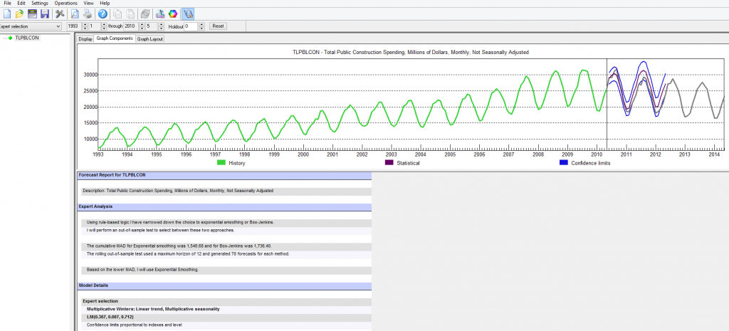
Here’s what the program panel looks like, after you trigger the automatic forecasting procedure (click to enlarge).

FPro

So basically you see a graph of the historic data you are feeding into the program. If you look down to Model Details you will see that expert selection picked a multiplicative Winters linear trend, multiplicative seasonality model. The estimated parameters are then given.

Above this, under Expert Analysis, the screen tells you that it looked at both Box-Jenkins (ARIMA) and ES models, picking the ES model based on out-of-sample tests.

Further down on this screen (not shown), the program lists the forecasts, which are graphed with confidence intervals above (shown).

I’ll discuss these forecasts, but first let me say a few words about the Hyndman R Forecast package analysis.

The Hyndman R Forecast Package

R is very big in some of the enterprise IT outfits. I have friends, for example, who view it as essential, and who have helped me recently come up to speed, to an extent, in using it.

After some fumbling around, I settled on running my R programs in R Studio. There is something called the Comprehensive R Archive Network (CRAN) with important open source R programs. Hyndman et al have their Forecast program listed there, and it pops up in R Studio, which is hugely convenient.

Again, there is an issue of data input. In this case, correctly positioning a csv spreadsheet file works well.

The R code I used to generate ES forecasts is as follows:

R

Note I screw up the spelling of ExponentialSmooth in naming the subdirectory. Oh well.

So after you import the csv file with the read command, you convert it to a time series format. Then, you can apply the operation ets(.) to the time series file, producing the parameters of the optimal ES model, based on comparisons of Akaike information criteria from the maximum likelihood estimations used to calculate the parameters of all the models.

Forecast selects ETS(M,Ad,M) as the optimal model. This indicates an additive trend is used, but is damped, and that the seasonal effects are multiplicative – more or less as in the Forecast Pro analysis.

The Forecasts

I called for 24 months of forecasts from both programs.

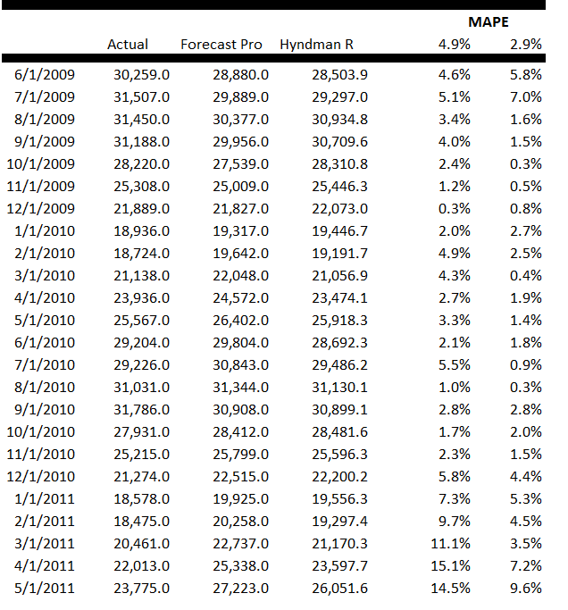
Here is a table comparing the forecasts from both packages with the actual values of this public construction time series.

TableFPH

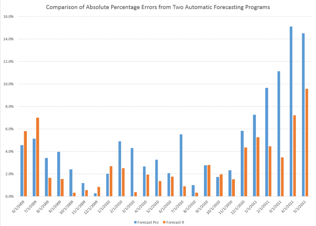
The Hyndman et al R Forecast package produces significantly lower Mean Absolute Percentage Error (MAPE) than Forecast Pro in these forecasts – 2.9% compared with 4.9%.

Here is a chart comparing the absolute percent error by month over the forecast horizon.

compRFP

Conclusions

This particular example is a case of random selection. I really have not run other forecasts with this data and these two models, except for actual future projections. So it’s interesting that an explicitly damped linear trend applied to these data generates a superior forecast to whatever it is that Forecast Pro does.

But readers should be aware that, in many instances, Forecast Pro can slightly outperform the R Forecast program, as Hyndman and coauthors document in a critical paper on this automatic forecasting setup in R.

However, the performance of the two programs is very similar.

In general, I would suggest that non-mathematical users, or folks not used to developing computer programs, stick with Forecast Pro, probably getting the company or organization you work for to pony up several hundred to several thousand dollars to get what you need for the scale of the forecasting problem at hand. Incidentally, I should be getting commissions for boosting this program, as often as I do, but I have no connection with the company.

For more mathematically sophisticated users, I strongly recommend getting up to speed on the R Forecast package and other R packages.

Both would be nice to use together. The R programs can support an interesting research effort, doing all sorts of clever things like fitting splines to the data, boosting, and bagging. Forecast Pro on the other hand is great if you have to produce a large number of forecasts and do not have time to dwell too much on the details of each series.

Exponential Smoothing – I

As I wrote recently, most business forecasting assignments are relatively simple. You collect the data (often the most challenging part), and plug this data into an automatic forecasting program. The program probably applies some type of exponential smoothing (ES) to produce forecasts for a horizon of a few periods ahead, and, bam, there you have it. The rest is presentation, developing the “story” and so forth.

So what about this exponential smoothing? What’s basically involved? What are the differences between exponential smoothing and the other primary univariate forecasting technique – ARIMA or Box-Jenkins modeling? What are these automatic forecasting programs, and which ones are best?

All good questions, and, if you are interested or involved in forecasting, the answers are good to rehearse from time to time.

Level, Trend, Seasonality – Components of Time Series

Exponential smoothing originated with the work of Brown and Holt for the US Navy (see the discussion in Gardiner). The perspective was not theoretical, but applied.

Nevertheless, there is an intuitive aspect to exponential smoothing (ES). That has to do with the decomposition of time series into components – such as level, trend, and seasonal effects.

So, applying the algorithms of ES to some time series Xt t=1,2,…,n, we extract estimates of the level Lt, trend Tt, and seasonal component, St, so that at any time t, we can express Xt as

Xt = Lt + Tt + St

This would be an additive model.

It’s also possible that the time series Xt could be multiplicative, as in

Xt = LtTtSt

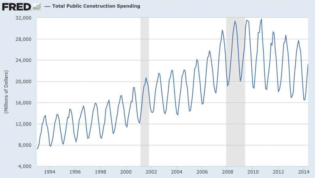
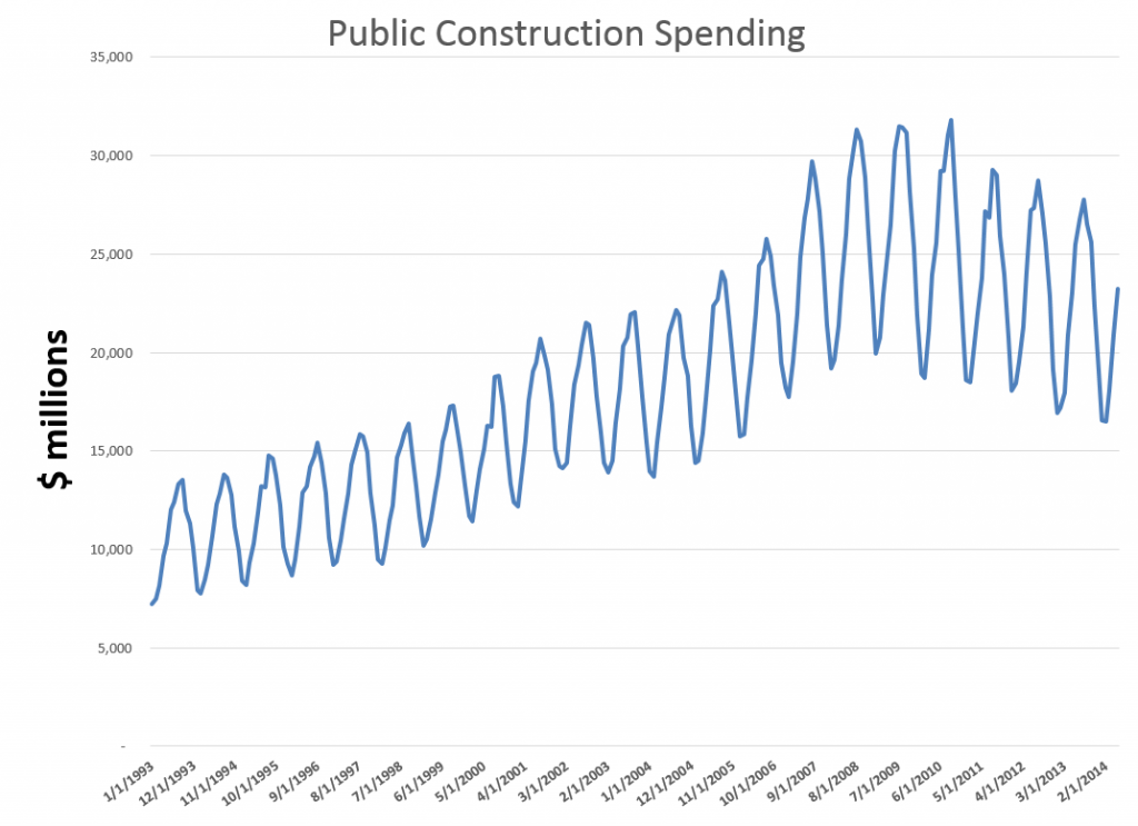
By way of example, consider the following time series for public construction spending in the US, obtained from FRED (Federal Reserve Economic Data).

PCS

Now if you look closely, it’s clear there are strongly delineated seasonal effects. Furthermore, these seasonal variations appear to fluctuate more or less in proportion to the annual levels of the series. Thus, the variation is considerably more over a year, when spending is at a $25 billion level, than it does at a $10 billion level.

And the fact that these levels are different, and the series does not simply oscillate around a single level, indicates that there is probably a meaningful trend component to this time series.

Automatic Forecasting Programs

These are the considerations that you take into account in building an exponential smoothing model.

Now it is possible to create ES models within the framework of a spreadsheet. Thus, ES models have smoothing parameters which can be set by minimizing a squared sum of forecast errors over historic data. In Microsoft’s Excel, you can use Solver to do this, once you set up the recursion equations for level, trend, and seasonal components or effects.

In coming posts, I want to show how this can be done for a simple example.

But really, setting up spreadsheets to estimate exponential smoothing models can be laborious, since you need a separate set of computations for every possible model. In addition to the additive and purely multiplicative models shown above, for example, there can be hybrid cases – multiplicative seasonality but additive trend, and so forth.

So it’s a good idea to equip yourself with one of the several, good automatic forecasting programs out there to speed model identification and evaluation.

I will have reference to two such automatic forecasting programs in coming posts – Forecast Pro and Rob Hyndman’s Forecast package in R. I’ll make comparisons between these programs. A demo version of Forecast Pro is available for download for free, but it is a commercial package with various options at various price steps. Hyndman’s R forecasting package, on the other hand, is open source software and free, as is the R platform. While this sounds like an unbeatable advantage, there always are questions of bugs and performance – which in this case seem to be to be resolved for reasons we can discuss.

What’s The Big Deal?

Finally, the reason why ES forecasting is so widely applied is that, in many cases, it produces forecasts which are of comparable or superior accuracy to other univariate forecasting approaches.

ES has performed well, for example, in international forecasting competitions, including the widely-publicized M-competitions.

There also is a link between exponential smoothing and the Kalman filter. So ES is in a sense an adaptive forecasting approach. For example, ES weights more recent observations more heavily than observations more distant in the past, unlike a regression trend model.

Finally, recent research has provided statistical pedigree to exponential smoothing, rescuing it in a sense from consignment to “a purely ad hoc” approach. Thus, there is a direct link between time series that embody a random walk or random walk with drift and exponential smoothing.

The Laplace Distribution and Financial Returns

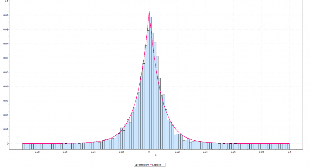
Well, using EasyFit from Mathwave, I fit a Laplace distribution to the residuals of the regression on S&P daily returns I discussed yesterday.

Here is the result.

Laplacefit

This beats a normal distribution hands down. It also appears to beat the Matlab fit of a t distribution, but I have to run down more details on forms of the t-distribution to completely understand what is going on in the Matlab setup.

Note that EasyFit is available for a free 30-day trial download. It’s easy to use and provides metrics on goodness of fit to make comparisons between distributions.

There is a remarkable book online called The Laplace Distribution and Generalizations. If you have trouble downloading it from the site linked here, Google the title and find the download for a free PDF file.

This book, dating from 2001, runs to 458 pages, has a good introductory discussion, extensive mathematical explorations, as well as applications to engineering, physical science, and finance.

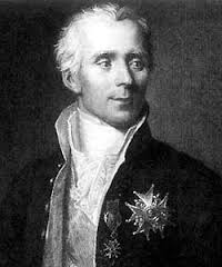
The French mathematical genius Pierre Simon Laplace proposed the distribution named after him as a first law of errors when he was 25, before his later discussions of the normal distribution.

The normal probability distribution, of course, “took over” – in part because of its convenient mathematical properties and also, probably, because a lot of ordinary phenomena are linked with Gaussian processes.

John Maynard Keynes, the English economist, wrote an early monograph (Keynes, J.M. (1911). The principal averages and the laws of error which lead to them, J. Roy. Statist. Soc. 74, New Series, 322-331) which substantially focuses on the Laplace distribution, highlighting the importance it gives to the median, rather than average, of sample errors.

The question I’ve struggled with is “why should stock market trading, stock prices, stock indexes lead, after logarithmic transformation and first differencing to the Laplace distribution?”

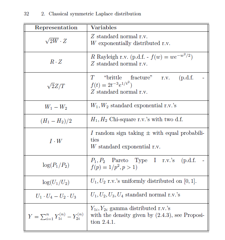
Of course, the Laplace distribution can be generated as a difference of exponential distributions, or as combination of a number of distributions, as the following table from Kotz, Kozubowski, and Podgorski’s book shows.

Ltable

This is all very suggestive, but how can it be related to the process of trading?

Indeed, there are quite a number of questions which follow from this hypothesis – that daily trading activity is fundamentally related to a random component following a Laplace distribution.

What about regression, if the error process is not normally distributed? By following the standard rules on “statistical significance,” might we be led to disregard variables which are drivers for daily returns or accept bogus variables in predictive relationships?

Distributional issues are important, but too frequently disregarded.

I recall a blog discussion by a hedge fund trader lamenting excesses in the application of the Black-Scholes Theorem to options in 2007 and thereafter.

Possibly, the problem is as follows. The residuals of autoregressions on daily returns and their various related transformations tend to cluster right around zero, but have big outliers. This clustering creates false confidence, making traders vulnerable to swings or outliers that occur much more frequently than suggested by a normal or Gaussian error distribution.

More on Automatic Forecasting Packages – Autobox Gold Price Forecasts

Yesterday, my post discussed the statistical programming language R and Rob Hyndman’s automatic forecasting package, written in R – facts about this program, how to download it, and an application to gold prices.

In passing, I said I liked Hyndman’s disclosure of his methods in his R package and “contrasted” that with leading competitors in the automatic forecasting market space –notably Forecast Pro and Autobox.

This roused Tom Reilly, currently Senior Vice-President and CEO of Automatic Forecast Systems – the company behind Autobox.

62_tom

Reilly, shown above, wrote  –

You say that Autobox doesn’t disclose its methods.  I think that this statement is unfair to Autobox.  SAS tried this (Mike Gilliland) on the cover of his book showing something purporting to a black box.  We are a white box.  I just downloaded the GOLD prices and recreated the problem and ran it. If you open details.htm it walks you through all the steps of the modeling process.  Take a look and let me know your thoughts.  Much appreciated!

AutoBox Gold Price Forecast

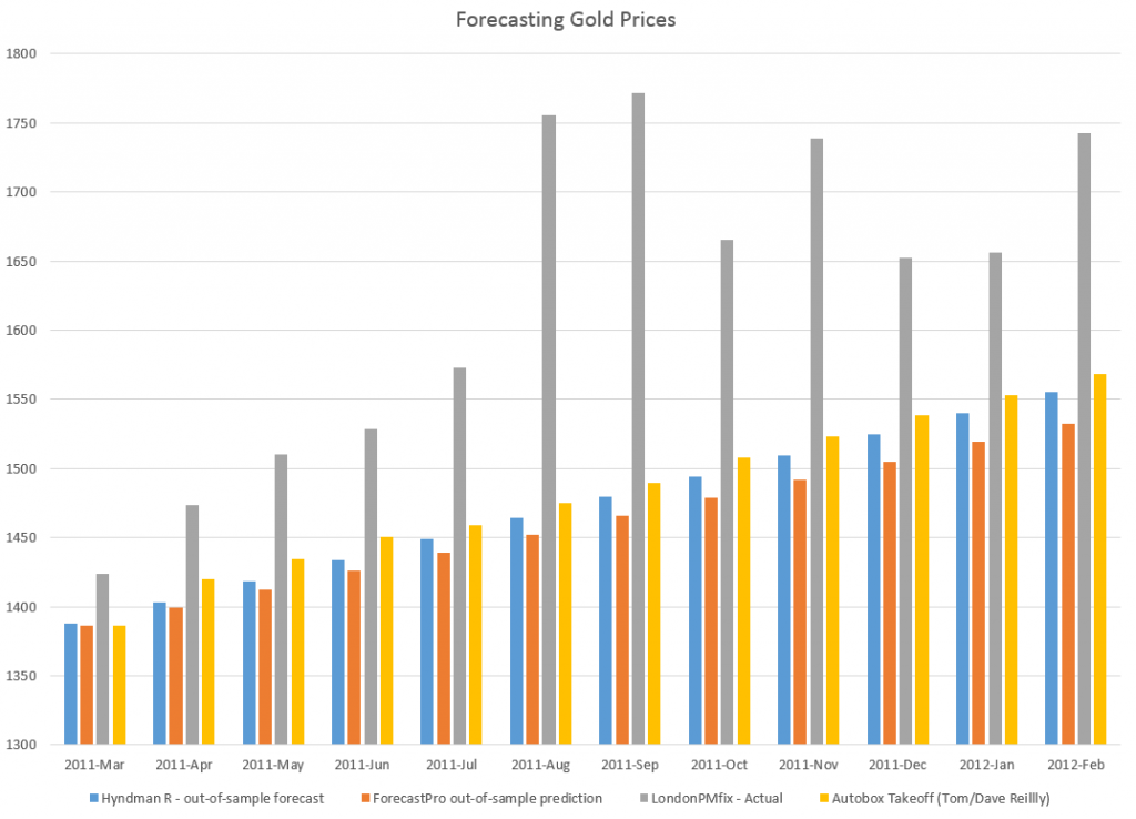
First, disregarding the issue of transparency for a moment, let’s look at a comparison of forecasts for this monthly gold price series (London PM fix).

A picture tells the story (click to enlarge).

ABFPHcomp

So, for this data, 2007 to early 2011, Autobox dominates. That is, all forecasts are less than the respective actual monthly average gold prices. Thus, being linear, if one forecast method is more inaccurate than another for one month, that method is less accurate than the forecasts generated by this other approach for the entire forecast horizon.

I guess this does not surprise me. Autobox has been a serious contender in the M-competitions, for example, usually running just behind or perhaps just ahead of Forecast Pro, depending on the accuracy metric and forecast horizon. (For a history of these “accuracy contests” see Markridakis and Hibon’s article on M3).

And, of course, this is just one of many possible forecasts that can be developed with this time series, taking off from various ending points in the historic record.

The Issue of Transparency

In connection with all this, I also talked with Dave Reilly, a founding principal of Autobox, shown below.

DaveReilly

Among other things, we went over the “printout” Tom Reilly sent, which details the steps in the estimation of a final time series model to predict these gold prices.

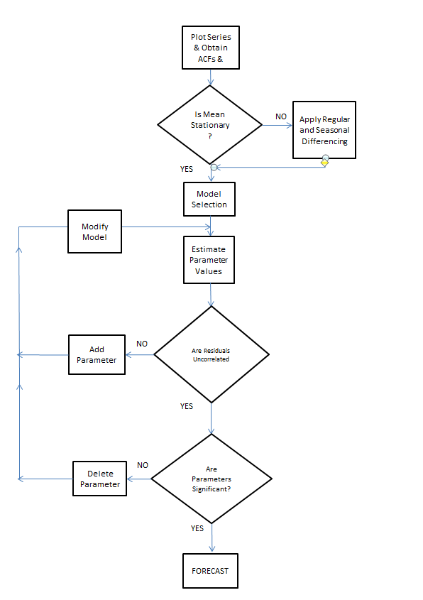
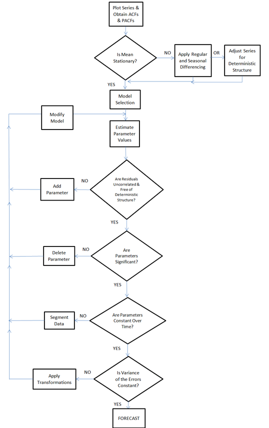
A blog post on the Autobox site is especially pertinent, called Build or Make your own ARIMA forecasting model? This discussion contains two flow charts which describe the process of building a time series model, I reproduce here, by kind permission.

The first provides a plain vanilla description of Box-Jenkins modeling.

Rflowchart1

The second flowchart adds steps revised for additions by Tsay, Tiao, Bell, Reilly & Gregory Chow (ie chow test).

Rflowchart2

Both start with plotting the time series to be analyzed and calculating the autocorrelation and partial autocorrelation functions.

But then additional boxes are added for accounting for and removing “deterministic” elements in the time series and checking for the constancy of parameters over the sample.

The analysis run Tom Reilly sent suggests to me that “deterministic” elements can mean outliers.

Dave Reilly made an interesting point about outliers. He suggested that the true autocorrelation structure can be masked or dampened in the presence of outliers. So the tactic of specifying an intervention variable in the various trial models can facilitate identification of autoregressive lags which otherwise might appear to be statistically not significant.

Really, the point of Autobox model development is to “create an error process free of structure.” That a Dave Reilly quote.

So, bottom line, Autobox’s general methods are well-documented. There is no problem of transparency with respect to the steps in the recommended analysis in the program. True, behind the scenes, comparisons are being made and alternatives are being rejected which do not make it to the printout of results. But you can argue that any commercial software has to keep some kernel of its processes proprietary.

I expect to be writing more about Autobox. It has a good track record in various forecasting competitions and currently has a management team that actively solicits forecasting challenges.

Loess Seasonal Decomposition as a Forecasting Tool

I’ve applied something called loess decomposition to the London PM Fix gold series previously discussed in this blog.

This suggests insights missing from an application of Forecast Pro – a sort of standard in the automatic forecasting field.

Loess decomposition separates a time series into components – trend, seasonals, and residuals or remainder – based on locally weighted regression smoothing of the data.

I always wondered whether, in fact, there was a seasonal component to the monthly London PM fix time series.

Not every monthly or quarterly time series has credible seasonal components, of course.

The proof would seem to be in the pudding. If a program derives seasonal components for a time series, do those seasonal components improve forecasts? That seems to be the critical issue.

STL Decomposition

STL decomposition – seasonal trend decomposition based on loess – was proposed by Cleveland et al in an interesting-sounding publication called “The Journal of Official Statistics.” I found the citation working through the procedure for bagging exponential smoothing mentioned in the previous post.

Amazingly, there is an online resource which calculates this loess decomposition for data you input, based on a listed R routine. The citation is Wessa P., (2013), Decomposition by Loess (v1.0.2) in Free Statistics Software (v1.1.23-r7), Office for Research Development and Education, URL http://www.wessa.net/rwasp_decomposeloess.wasp/

Comparison of STL Decomposition and Forecast Pro Gold Price Forecasts

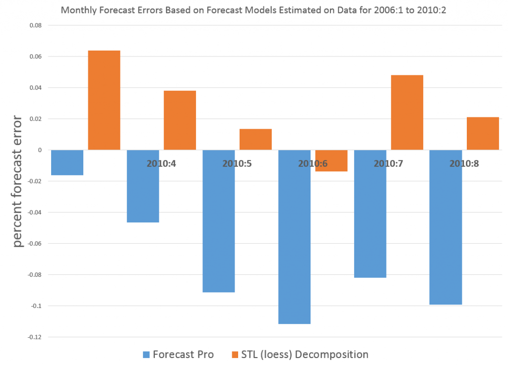
Here’s a typical graph comparing the forecast errors from the Forecast Pro runs with STL Decomposition.

goldloessFP

The trend component extracted by the STL decomposition was uncomplicated and easy to forecast by linear extrapolation. I added the seasonal component to these extrapolations to get the monthly forecasts over the six month forecast horizon. Forecast Pro, on the other hand, did not signal the existence of a seasonal component in this series, and, furthermore, identified the optimal forecast model as a random walk and the optimal forecast as the last observed value.

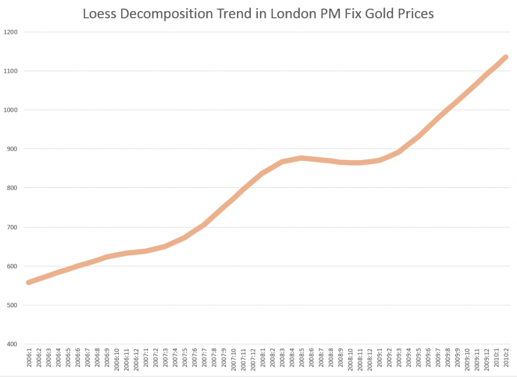
Here is the trend component from the STL decomposition.

Goldtrend

Discussion

Potentially, there is lots more to discuss here.

For example, to establish forecasts based on the loess decomposition of the gold price outperform Forecast Pro means compiling a large number of forecast comparisons, ideally one for all possible training sets beyond a minimum number of observations required for stable calculation of the STL algorithm. That is, each training set generates somewhat different values for the trend, seasonals, and residuals with loess decomposition. And Forecast Pro needs to be run for all these possible training sets also, with forecasts compared to out-of-sample data.

While I have not gone to this extent, I have done these computations several times with good results for STL decomposition.

Also, it’s clear that loess decomposition extracts constant variance seasonals. However, the shape of these seasonals change as the training set changes. It is necessary, thus, to study whether these changes can reflect multiplicative seasonality, for series in which that type of seasonality predominates. For example, perhaps STL seasonals tend to reflect the end points of the training sets.

Bergmeir, Hyndman, and Benıtez (BHB) apply a Box Cox transformation in one of their bagged exponential smoothing methods. This is possibly another way to sidestep problems of multiplicative or hetereoskedastic seasonality. It also makes sense when one is attempting to bag a time series.

However, my explorations suggest the results of STL decomposition are quite flexible, and, in the case of this gold price series, often produce superior forecasts to results from one of the main off-the-shelf automatic forecasting programs.

I personally am going to work on including STL decomposition in my forecasting toolkit.

Links – February 28

Data Science and Predictive Analytics

Data Scientists Predict Oscar® Winners Again; Social Media May Love Leo, But Data Says “No”

..the data shows that Matthew McConaughey will win best actor for his role in the movie Dallas Buyers Guide; Alfonso Cuaron will win best director for the movie Gravity; and 12 Months a Slave will win the coveted prize for best picture – which is the closest among all the races. The awards will not be a clean sweep for any particular picture, although the other award winners are expected to be Jared Leto for best supporting actor in Dallas Buyers Club; Cate Blanchet for best actress in Blue Jasmine; and Lupita Nyong’o for best supporting actress in 12 Years a Slave.

10 Most Influential Analytics Leaders in India

Pankaj Kulshreshtha – Business Leader, Analytics & Research at Genpact

Rohit Tandon – Vice President, Strategy WW Head of HP Global Analytics

Sameer Dhanrajani – Business Leader, Cognizant Analytics

Srikanth Velamakanni – Co founder and Chief Executive Officer at Fractal Analytics

Pankaj Rai – Director, Global Analytics at Dell

Amit Khanna – Partner at KPMG

Ashish Singru – Director eBay India Analytics Center

Arnab Chakraborty – Managing Director, Analytics at Accenture Consulting

Anil Kaul – CEO and Co-founder at Absolutdata

Dr. N.R.Srinivasa Raghavan, Senior Vice President & Head of Analytics at Reliance Industries Limited

Interview with Jörg Kienitz, co-author with Daniel Wetterau of Financial Modelling: Theory, Implementation and Practice with MATLAB Source

JB: Why MATLAB? Was there a reason for choosing it in this context?

JK: Our attitude was that it was a nice environment for developing models because you do not have to concentrate on the side issues. For instance, if you want to calibrate a model you can really concentrate on implementing the model without having to think about the algorithms doing the optimisation for example. MATLAB offers a lot of optimisation routines which are really reliable and which are fast, which are tested and used by thousands of people in the industry. We thought it was a good idea to use standardised mathematical software, a programming language where all the mathematical functions like optimisation, like Fourier transform, random number generator and so on, are very reliable and robust. That way we could concentrate on the algorithms which are necessary to implement models, and not have to worry about a programming a random number generator or such stuff. That was the main idea, to work on a strong ground and build our house on a really nice foundation. So that was the idea of choosing MATLAB.

Knowledge-based programming: Wolfram releases first demo of new language, 30 years in the making


Economy

Credit Card Debt Threatens Turkey’s Economy – kind of like the subprime mortgage scene in the US before 2008.

..Standard & Poor’s warned in a report last week that the boom in consumer credit had become a serious risk for Turkish lenders. Slowing economic growth, political turmoil and increasing reluctance by foreign investors to provide financing “are prompting a deterioration in the operating environment for Turkish banks,”

A shadow banking map from the New York Fed. Go here and zoom in for detail.

China Sees Expansion Outweighing Yuan, Shadow Bank Risk

China’s Finance Minister Lou Jiwei played down yuan declines and the risks from shadow banking as central bank Governor Zhou Xiaochuan signaled that the nation’s economy can sustain growth of between 7 percent and 8 percent.

Outer Space

715 New Planets Found (You Read That Number Right)

Speaks for itself. That’s a lot of new planets. One of the older discoveries – Tau Boötis b – has been shown to have water vapor in its atmosphere.

Hillary, ‘The Family,’ and Uganda’s Anti-Gay Christian Mafia

GayBashers

I heard about this at the SunDance film gathering in 2013. Apparently, there are links between US and Ugandan groups in promulgating this horrific law.

An Astronaut’s View of the North Korean Electricity Black Hole

NorthKorea