Big Data, energy forecasting, technology forecasting

Big Data and Fracking

December 9, 2014 Clive Jones

Texas’ Barnett Shale, shown below, is the focus of recent Big Data analytics conducted by the Texas Bureau of Economic Geology.

The results provide, among other things, forecasts of when natural gas production from this field will peak – suggesting at current prices that peak production may already have been reached.

The Barnett Shale study examines production data from all individual wells drilled 1995-2010 in this shale play in the Fort Worth basin – altogether more than 15,000 wells.

Well-by-well analysis leads to segmentation of natural gas and liquid production potential in 10 productivity tiers, which are then used to forecast future production.

Decline curves, such as the following, are developed for each of these productivity tiers. The per-well production decline curves were found to be inversely proportional to the square root of time for the first 8-10 years of well life, followed by exponential decline as what the geologists call “interfracture interference” began to affect production.

A write-up of the Barnett Shale study by its lead researchers is available to the public in two parts at the following URL’s:

http://www.beg.utexas.edu/info/docs/OGJ_SFSGAS_pt1.pdf

http://www.beg.utexas.edu/info/docs/OGJ_SFSGAS_pt2.pdf

Econometric analysis of well production, based on porosity and a range of other geologic and well parameters is contained in a followup report Panel Analysis of Well Production History in the Barnett Shale conducted under the auspices of Rice University.

Natural Gas Production Forecasts

Among the most amazing conclusions for me are the predictions regarding total natural gas production at various prices, shown below.

This results from a forecast of field development (drilling) which involved a period of backcasting 2011-2012 to calibrate the BEG economic and production forecast models.

Essentially, it this low price regime continues through 2015, there is a high likelihood we will see declining production in the Barnett field as a whole.

Of course, there are other major fields – the Bakken, the Marcellus, the Eagle-Ford, and a host of smaller, newer fields.

But the Barnett Shale study provides good parameters for estimating EUR (estimate ultimate recovery) in these other fields, as well as time profiles of production at various prices.

energy forecasting, technology forecasting

Forecasting Shale Oil/Gas Decline Rates

December 8, 2014 Clive Jones 1 Comment

Forecasting and data analytics increasingly are recognized as valued partners in nonconventional oil and gas production.

Fracking and US Oil/Gas Production

“Video Friday” here presented a YouTube with Brian Ellis – a Michigan University engineer – discussing hydraulic fracturing and horizontal drilling (“fracking”).

Fracking produced the hockey stick at the end of this series.

These new technologies also are responsible for a bonanza of natural gas, so much that it often has nowhere to go – given the limited pipeline infrastructure and LNG processing facilities.

Rapid Decline Curves for Fracking Oil and Gas

In contrast to conventional wells, hydraulic fracturing and horizontal drilling (“fracking”) produces oil and gas wells with rapid decline curves.

Here’s an illustration from the Penn State Department of Energy and Mineral Engineering site,

The two legends at the bottom refer to EUR’s– estimated ultimate recovery times (click to enlarge).

Conventional oil fields typically have decline rates on the order of 5 percent per year.

Shale oil and gas wells, on the other hand, may produce 50 percent or more of their total EUR in their first year of operation.

There are physical science fundamentals behind this, explained, for example, in

Decline and depletion rates of oil production: a comprehensive investigation

You can talk, for example, of shale production being characterized by a Transient Flow Period followed by Boundary Dominated Flow (BDF).

And these rapid decline rates have received a lot of recent attention in the media:

Could The ‘Shale Oil Miracle’ Be Just A Pipe Dream?

Wells That Fizzle Are a ‘Potential Show Stopper’ for the Shale Boom

Is the U.S. Shale Boom Going Bust?

Forecasting and Data Analytics

One forecasting problem in this context, therefore, is simply to take histories from wells and forecast their EUR’s.

Increasingly, software solutions are applying automatic fitting methods to well data to derive decline curves and other shale oil and gas field parameters.

Here is an interesting product called Value Navigator.

This whole subject is developing rapidly, and huge changes in the US industry are expected, if oil and gas prices continue below $60 a barrel and $4 MMBtu.

The forecasting problem may shift from well and oil field optimization to evaluation of the wider consequences of recent funding of the shale oil and gas boom. But, again, the analytics are available to do this, to a large extent, and I want to post up some of what I have discovered in this regard.

ensemble forecasts, technology forecasting

Video Friday – Fracking

December 5, 2014 Clive Jones

Here is Brian Ellis from Michigan University Engineering with a look at the technology of hydraulic fracturing (fracking) and horizontal drilling – the innovations that recently pushed US oil production near the 10 million barrel per day mark.

I’m putting this up, rather than other, often excellent film clips showing people lighting water from their kitchen taps because the scale of shale oil and gas production has become so large. There really is a huge tradeoff between current employment and business activity and long term environmental effects.

Price, rather than environmental concerns, are likely to be the crucial factor in any scaleback.

At the same time, there is the possibility of further technical advance in the US shale oil and gas technologies, advances which may push extraction prices lower, giving the industry a longer lease during what may be a year or more of lower oil prices.

Fracking and its possible dynamics are critical to a lot of business activity and, thus, forecasting in the US.

Chinese economy, forecasting research, forecasting trade balances

China – Trade Colossus or Assembly Site?

December 4, 2014 Clive Jones

There is a fascinating paper – How the iPhone Widens the United States Trade Deficit with the People’s Republic of China. In this Asian Bank Development Institute (ADBI) white paper, Yuqing Ying and his coauthor document the value chain for an Apple iPhone:

The source for this breakout, incidentally, is a “teardown” performed by the IT market research company iSupply, still accessible at –https://technology.ihs.com/389273/iphone-3g-s-carries-17896-bom-and-manufacturing-cost-isuppli-teardown-reveals. In other words, iSupply physically took apart an iPhone to identify the manufacturers of the components.

The Paradox

After estimating that, in

2009 iPhones contributed US$1.9 billion to the trade deficit, equivalent to about 0.8% of the total US trade deficit with the PRC,

the authors go on to point out that

..most of the export value and the deficit due to the iPhone are attributed to imported parts and components from third countries and have nothing to do with the PRC. Chinese workers simply put all these parts and components together and contribute only US$6.5 to each iPhone, about 3.6% of the total manufacturing cost (e.g., the shipping price). The traditional way of measuring trade credits all of the US$178.96 to the PRC when an iPhone is shipped to the US, thus exaggerating the export volume as well as the imbalance. Decomposing the value added along the value chain of iPhone manufacturing suggests that, of the US$2.0 billion worth of iPhones exported from the PRC, 96.4% in fact amounts to transfers from Germany (US$326 million), Japan (US$670 million), Korea (US$259 million), the US (US$108 million), and other countries (US$ 542 million). All of these countries are involved in the iPhone production chain.

Yuqing Xing builds on the paradox in his more recent China’s High-Tech Exports: The Myth and Reality published in 2014 in MIT’s Asian Economic Papers.

Prevailing trade statistics are inconsistent with trade based on global supply chains and mistakenly credit entire values of assembled high-tech products to China. China’s real contribution to the reported 82 percent high-tech exports is labor not technology. High-tech products, mainly made of imported parts and components, should be called “Assembled High-tech.” To accurately measure high-tech exports, the value-added approach should be utilized with detailed analysis on the value chains distributions across countries. Furthermore, if assembly is the only source of value-added by Chinese workers, in terms of technological contribution these assembled high-tech exports are indifferent to labor-intensive products, and so they should be excluded from the high-tech classification.

MNEs, in particular Taiwanese IT firms in China, have performed an important role in the rapid expansion of high-tech exports. The trend of production fragmentation and outsourcing activities of MNEs in information and communication technology has benefitted China significantly, because of its huge labor endowment. The small share of indigenous firms in high-tech exports implies that China has yet to become a real competitor of the United States, EU, and Japan. That China is the number one high-tech exporter is thus a myth rather than a reality.

Ying and Yang

This perspective – that it is really “value-added” that we should focus on, rather than the total dollar volume of trade coming in or going out of a country – is interesting, but I can’t help but think there is a disconnect when you consider actual Chinese foreign exchange reserves, shown below (source – http://www.stats.gov.cn/tjsj/ndsj/2013/indexeh.htm).

So currently China holds nearly 3.5 trillion dollars in foreign exchange reserves – most of which, but not all, is comprised of US dollars.

This is a huge amount of money, on the order of five percent of total global GDP.

How could China have accumulated this merely by being an assembly site for high tech and other products (see Five Facts about Value-Added Exports and Implications for Macroeconomics and Trade Research)? How can this be attributable just to mistakes in counting the origin of the many components in goods coming from China? Don’t those products have to come in and be counted as imports?

There is a mystery here, which it would be good to resolve.

Assembly photo at top from Apple Insider

Chinese economy, global business forecasts, purchasing power parity

China Passes US in Terms of Purchasing Power Parity

November 30, 2014 Clive Jones

The International Monetary Fund (IMF) announced recently that Chinese GDP passed that of the United States – in terms of purchasing power parity (PPP).

Business Insider charts the relative sizes of the Chinese and US economies in terms of total global output, where, again, production is measured in terms of purchasing power output.

According to the World Bank,

Purchasing power parity conversion factor is the number of units of a country’s currency required to buy the same amount of goods and services in the domestic market as a U.S. dollar would buy in the United States.

In a less serious vein, the Economist magazine maintains the Big Mac Index. This is informative, however, inasmuch as MacDonalds outlets range across the globe.

In July of this year, the Economist lists the US price of a Big Mac hamburger as $4.80.

China is among the cheapest places to buy a Big Mac, as shown in this table from Economist data.

The China Big Mac Index, therefore, is 0.57, suggesting Chinese yuan purchase almost twice the actual goods and services in China, as their dollar exchange rate would suggest.

Or to do this calculation based on the current exchange rate, 1 US dollar buys 6.41 Chinese 1 yuan.

So, if the local price has not changed, 16.9 yuan buy a Big Mac, indicating that a Big Mac now has a dollar price of $2.63. Then, if today’s Big Mac still costs $4.80, the renmimbi buys 4.8/2.63 or 1.83 times as much as its market exchange rate indicates. Hence, according to a Big Mac type index evaluation, the renmimbi is undervalued.

This is a pretty good calculation, according to the World Bank, which lists the conversion factor as 0.7.

Of course, there are four to five times as many residents of the People’s Republic of China, as there are US residents. Per capita Chinese incomes, accordingly, are four to five times lower, even in terms of purchasing power parity.

And in terms of market exchange values, the IMF estimates 2014 Chinese GDP at 10,355 billion dollars, compared with $17,416 billion for the US.

The rise of Chinese production has been truly spectacular, as this chart of Chinese GDP shows, based on official Chinese statistics.

There are a lot of other remarkable charts that can be pulled together about China, and I am planning several future posts along these lines.

See you this coming week!

Chinese official courtesy of Wikipedia

accuracy of forecasts, global business forecasts, predicting oil prices

Followup on OPEC and the Price of Oil

November 28, 2014 Clive Jones

Well, readers here may have noticed, Business Forecast Blog correctly predicted the OPEC decision about reducing oil production at their Thanksgiving Thursday (November 27) meeting in Vienna.

USA Today reports,

VIENNA — Crude prices plunged Thursday after the powerful Organization of Petroleum Exporting Countries said it wouldn’t cut production levels to stem the collapse in oil prices that have fallen 40% since June.

Saudi Arabia’s oil minister Ali Al-Naimi delivered the news as he left a nearly five-hour meeting of the cartel’s 12 oil ministers here.

Our post was called The Limits of OPEC and was studded with passages of deep foresight, such as

I’m kind of a contrarian here. I think the sound and fury about this Vienna meeting on Thanksgiving may signify very little in terms of oil prices – unless global (and especially Chinese) economic growth picks up. As the dominant OPEC producer, Saudi Arabia may have market power, but, otherwise, there is little evidence OPEC functions as a cartel. It’s hard to see, also, that the Saudi’s would unilaterally reduce their output only to see higher oil prices support US frackers continuing to increase their production levels at current rates.

The immediate response to the much-anticipated OPEC meeting was a plunge in the spot price of West Texas Intermediate (WTI) to below $70 a barrel.

Brent, the other pricing standard, fared a little better, but dropped significantly,

Both charts are courtesy of the Financial Times of London.

The Reuters article on the OPEC decision – Saudis block OPEC output cut, sending oil price plunging – is full of talk that letting prices drift lower, perhaps down to $60-65 a barrel, is motivated by a desire to wing higher-cost US producers, and also, maybe, to squeeze Russia and Iran – other players who are out of favor with Saudi Arabia and other Gulf oil states.

Forecasting Issues and Techniques

Advice – get the data, get the facts. Survey Bloomberg and other media by relevant news story and topic, but whenever possible, go to the source.

For example, lower oil prices may mean Saudi Arabia and some other Gulf oil states have to rely more on accumulated foreign exchange to pay their bills, since their lavish life-styles probably adjusted to higher prices (even though raw production costs may be as low as $25 a barrel). Just how big are these currency reserves, and can we watch them being drawn down? There is another OPEC meeting apparently scheduled for June 2015

Lead picture of Saudi Oil Minister from Yahoo.

Chinese economy, energy forecasting, global business forecasts

The Limits of OPEC

November 23, 2014 Clive Jones

There’s rampant speculation and zero consensus about the direction OPEC will take in their upcoming Vienna meeting, November 27.

Last Friday, for example. Bloomberg reported,

The 20 analysts surveyed this week by Bloomberg are perfectly divided, with half forecasting the Organization of Petroleum Exporting Countries will cut supply on Nov. 27 in Vienna to stem a plunge in prices while the other half expect no change. In the seven years since the surveys began, it’s the first time participants were evenly split. The only episode that created a similar debate was the OPEC meeting in late 2007, when crude was soaring to a record.

Many discussions pose the strategic choice as one between –

(a) cutting production to maintain prices, but at the cost of losing market share to the ascendant US producers, and

(b) sustaining current production levels, thus impacting higher-cost US producers (if the low prices last long enough), but risking even lower oil prices – through speculation and producers breaking ranks and trying to grab what they can.

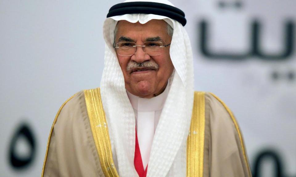
Lybia, Ecuador, and Venezuela are pushing for cuts in production. Saudi Arabia is not tipping its hand, but is seen by many as on the fence about reducing production.

OPEC Members, Production, and Oil Prices

The Organization of Petroleum Exporting Countries (OPEC) has twelve members, whose production over recent years is documented in the following table.

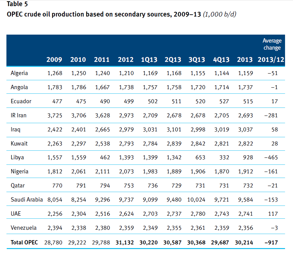
According to the OPEC Annual Report, global oil supply in 2013 ran about 90.2 mb/d, while, as the above table indicates, OPEC production was 30.2 mb/d. So OPEC provided 33.4 percent of global oil supplies in 2013 with Saudi Arabia being the largest producer – overwhelmingly.

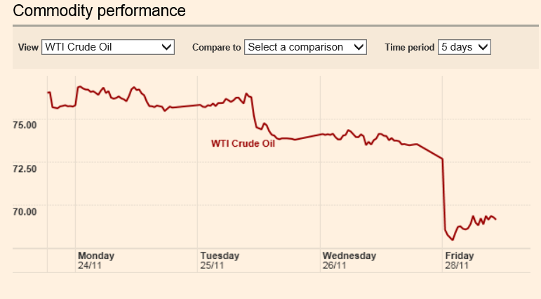
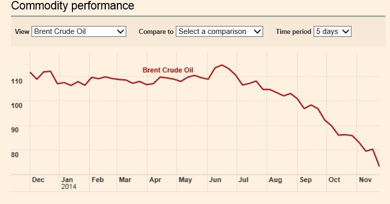
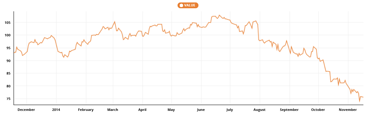
Oil prices, of course, have spiraled down toward $75 a barrel since last summer.

Is OPEC an Effective Cartel?

There is a growing literature questioning whether OPEC is an effective cartel.

This includes the recent OPEC: Market failure or power failure? which argues OPEC is not a working cartel and that Saudi Arabia’s ideal long term policy involves moderate prices guaranteed to assure continuing markets for their vast reserves.

Other recent studies include Does OPEC still exist as a cartel? An empirical investigation which deploys time series tests for cointegration and Granger causality, finding that OPEC is generally a price taker, although cartel-like features may adhere to a subgroup of its members.

The research I especially like, however, is by Jeff Colgan, a political scientist – The Emperor Has No Clothes: The Limits of OPEC in the Global Oil Market.

Colgan poses four tests of whether OPEC functions as a cartel -.

new members of the cartel have a decreasing or decelerating production rate (test #1); members should generally produce quantities at or below their assigned quota (test #2); changes in quotas should lead to changes in production, creating a correlation (test #3); and members of the cartel should generally produce lower quantities (i.e., deplete their oil at a lower rate) on average than non-members of the cartel (test #4)

Each of these tests fail, putting, as he writes, the burden of proof on those who would claim that OPEC is a cartel.

Here’s Colgan’s statistical analysis of cheating on the quotas.

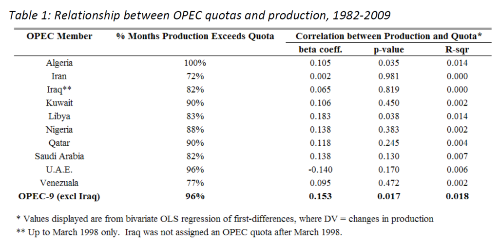
On average, he calculates that the nine principal members of OPEC produced 10 percent more oil than their quotas allowed – which is equivalent to 1.8 million barrels per day, on average, which is more than the total daily output of Libya in 2009.

Finally, there is the extremely wonkish evidence from academic studies of oil and gas markets more generally.

There are, for example, several long term studies of cointegration of oil and gas markets. These studies rely on tests for unit roots which, as I have observed, have low statistical power. Nevertheless, the popularity of this hypothesis seems to be consistent with very little specific influence of OPEC on oil production and prices in recent decades. The 1970’s may well be an exception, it should be noted.

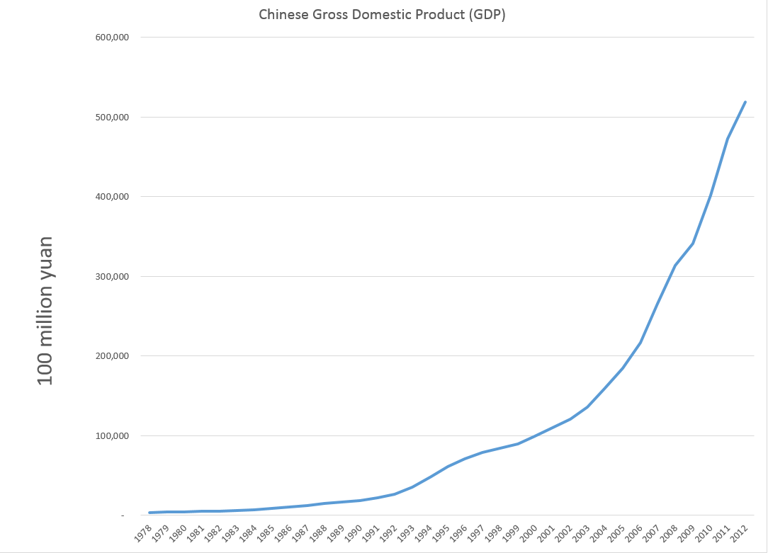
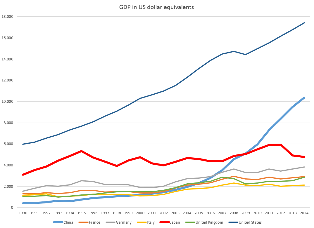
We will see in coming weeks. Or maybe not, since it still will be necessary to sort out influences such as quickening of the pace of economic growth in China with recent moves by the Chinese central bank to reduce interest rates and keep the bubble going.

If I were betting on this, however, I would opt for a continuation of oil prices below $100 a barrel, and probably below $90 a barrel for some time to come. Possibly even staying around $70 a barrel.

Japanese economy, macroeconomic forecasting

Some Thoughts on Japan

November 20, 2014 Clive Jones

I saw the news that Japan has fallen into recession again. This “hit the wires” just after the Bank of Japan surprised everyone and announced a major new quantitative easing (QE) program.

Japan is a country of 127 million persons (2013) with one of the largest economies in the world, as this chart shows.

Basically, though, the Japanese economy has been a start/stop mode since the mid-1990’s. According these GDP estimates, China surpassed Japan 2008-2009, and now in nominal terms has a production level twice that of Japan.

The data are from the World Economic Outlook database (IMF) and are not inflation-adjusted, but are converted into US dollar equivalents.

Where’s the Beef?

Well, a person In Kansas might say, “So what?” Why is Japan important?

I think there are several reasons.

First, a recession in Japan, because of its continuing economic size, has the capability of affecting global markets.

According to the CIA Factbook .. on a purchasing power parity (PPP) basis that adjusts for price differences, Japan in 2013 stood as the fourth-largest economy in the world after second-place China, which surpassed Japan in 2001, and third-place India, which edged out Japan in 2012.

Simultaneous recessions in Japan and Europe almost surely would trigger a global economic slowdown, unless the American consumer just went crazy.

Test Case for Macroeconomic Policy

Another reason Japan is important is as a sort of test case for macroeconomic policy, as well as for the impacts of an aging population.

This chart shows the intermittent economic growth in Japan since the 1990’s along with the deflationary trend.

These figures are developed from official Japanese statistics.

Notice that you could start at around 1999 and draw a trendline for the Japanese CPI to about 2013, where a brief period 2008-2009 would appear as a blip away from this trendline.

Deflation has been a twenty year phenomena in Japan, and the current government, under Abe, has sought to break its hold with a triple-threat of fiscal policy, monetary policy, and structural reform.

The result is a continuation of the climb in the liabilities to GDP ratio of the Bank of Japan (BOJ), as shown in this chart extracted from Bloomberg sources.

So “steady as she goes,” the monetary base of Japan will reach about 50 percent of Japanese GDP within a year or two. This compares with a figure of just less than 20 percent for the United States.

The swing into negative growth in 2014 was triggered by a substantial increase in the VAT or value-added tax in Japan, and there is vigorous debate about future increases – viz Krugman Japan on the Brink.

Structural Reform

I wonder whether it might be better to question the religion of economic growth, than to attempt “structural reform” aka reductions in the real wage.

In any case, it easy to see that the recent surge in Japanese inflation, combined with additional consumption taxes and, indeed, negative economic growth mean that Japanese real wages are being reduced in real time here. Indeed Edward Hugh documents this with reference to official Japanese statistics.

But this is a slippery slope.

On the one hand, reductions in the real wage could make domestically produced Japanese goods more competitive in international markets.

On the other hand, domestic purchasing power could suffer, or, at the least, there could be a move to increasing concentrations of wealth. We’ve certainly seen that in the United States, where the real wage of workers has declined off and on, since 1971, compensated for, to an extent, by the entry of women into the workforce and two-wage households.

The limits of human intellect can be found right here. The enormous production growth in China has been accompanied by choking air pollution which, I can assure you from personal experience, is simply amazingly bad sometimes. Health-threatening. Yet the Chinese naturally want to expand their productive apparatus to the extent they can, for purposes of providing for their vast population and in order to secure China’s place in the global economy.

But life in Japan – during these decades when economic growth has been very intermittent and prices have dropped – life has been fairly good. That’s one reason why many Japanese are now starting to enjoy their older years in a degree of relative comfort unimaginable one or two generations ago.

Maybe some Japanese visionary can come up with a sequel to Herman Daly’s steady state economy idea – a kind of reverse mortgage for an entire economy perhaps.

financial forecasts, stock market forecasts, time series forecasting

Quantitative Easing (QE) and the S&P 500

November 17, 2014 Clive Jones

Reading Jeff Miller’s Weighing the Week Ahead: Time to Buy Commodities 11/16/14 on Dash of Insight the following chart (copied from Business insider) caught my attention.

In the Business Insider discussion – There’s A Major Problem With The Popular Chart That Connects The Fed To The Stock Market – Myles Udland quotes an economist at Bank of America Merrill Lynch who says,

“Implicitly, this chart assumes that the markets are not forward looking and it is the implementation of Q that drives the stock market: when the Fed buys, the market booms and when it stops, the market swoons..”

“As our readers know [Ethan Harris of Bank of America Merrill Lynch writes] we think this relationship is a classic case of spurious correlation: anything that trended higher over the last 5 years has a 90%-plus correlation with the Fed’s balance sheet.”

This makes a good point inasmuch as two increasing time series can be correlated, but lack any essential relationship to each other – a condition known as “spurious correlation.”

But there’s more to it than that.

I am surprised that these commentators, all of whom are sophisticated with numbers, don’t explore one step further further and look at first differences of these time series. Taking first differences turns Fed liabilities and the S&P 500 into stationary series, and eliminates the possibility of spurious correlation in the above sense.

I’ve done some calculations.

Before reporting my results, let me underline that we have to be talking about something unusual in time, as this chart indicates.

Clearly, if there is any determining link between these monthly data for the monetary base (downloaded from FRED) and monthly averages for the S&P 500, it has be to after sometime in 2008.

In the chart above and in my computations, I use St. Louis monetary base data as a proxy for the Fed liabilities series in the Business Insider discussion,

So then considering the period from January 2008 to the present, are there any grounds for claiming a relationship?

Maybe.

I develop a “bathtub” model regression, with 16 lagged values of the first differences of the monetary base numbers to predict the change in the month-to-month change in the S&P 500. I use a sample from January 2008 to December 2011 to estimate the first regression. Then, I forecast the S&P 500 on a one-month-ahead basis, comparing the errors in these projections with a “no-change” forecast. Of course, a no change forecast is essentially a simple random walk forecast.

Here are the average mean absolute percent errors (MAPE’s) from the first of 2012 to the present. These are calculated in each case over periods spanning January 2012’s MAPE to the month of the indicated average, so the final numbers on the far right of these lines are the averages for the whole period.

Lagged changes in the monetary base do seem to have some predictive power in this time frame.

But their absence in the earlier period, when the S&P 500 fell and rose to its pre-recession peak has got to be explained. Maybe the recovery has been so weak that the Fed QE programs have played a role this time in sustaining stock market advances. Or the onset of essentially zero interest rates gave the monetary base special power. Pure speculation.

Interesting, because it involves the stock market, of course, but also because it highlights a fundamental issue in statistical modeling for forecasting. Watch out for correlations in increasing time series. Always check first differences or other means of reducing the series to stationarity before trying regressions – unless, of course, you want to undertake an analysis of cointegration.

consumer behavior, Medical data analytics

Video Friday – Benefits and Risks of Alcoholic Drinks

November 14, 2014 Clive Jones

Like almost everyone who enjoys beer, wine, and mixed drinks, I have been interested in the research showing links between moderate alcohol consumption and cardiovascular health. In discussions with others, I’ve often heard, “now that’s the kind of scientific research we need more of” and so forth.

But obviously, booze is a two-edge sword.

So this research by Dr. James O’Keefe, a cardiologist from Mid America Heart Institute, with his co-authors Dr. Salman K. Bhatti, Dr. Ata Bajwa, James J. DiNicolantonio, Doctor of Pharmacy, and Dr. Carl J. Lavie caught my eye, because its comprehensive review of the literature on both benefits and risks.

It was published in the Mayo Clinic Proceedings, and here Dr. O’Keefe summarizing the findings.

The Abstract for this research paper, Alcohol and Cardiovascular Health: The Dose Makes the Poison…or the Remedy, lays it out pretty clearly.

Habitual light to moderate alcohol intake (up to 1 drink per day for women and 1 or 2 drinks per day for men) is associated with decreased risks for total mortality, coronary artery disease, diabetes mellitus, congestive heart failure, and stroke. However, higher levels of alcohol consumption are associated with increased cardiovascular risk. Indeed, behind only smoking and obesity, excessive alcohol consumption is the third leading cause of premature death in the United States. Heavy alcohol use (1) is one of the most common causes of reversible hypertension, (2) accounts for about one-third of all cases of nonischemic dilated cardiomyopathy, (3) is a frequent cause of atrial fibrillation, and (4) markedly increases risks of stroke—both ischemic and hemorrhagic. The risk-to-benefit ratio of drinking appears higher in younger individuals, who also have higher rates of excessive or binge drinking and more frequently have adverse consequences of acute intoxication (for example, accidents, violence, and social strife). In fact, among males aged 15 to 59 years, alcohol abuse is the leading risk factor for premature death. Of the various drinking patterns, daily low- to moderate-dose alcohol intake, ideally red wine before or during the evening meal, is associated with the strongest reduction in adverse cardiovascular outcomes. Health care professionals should not recommend alcohol to nondrinkers because of the paucity of randomized outcome data and the potential for problem drinking even among individuals at apparently low risk. The findings in this review were based on a literature search of PubMed for the 15-year period 1997 through 2012 using the search terms alcohol, ethanol, cardiovascular disease, coronary artery disease, heart failure, hypertension, stroke, and mortality. Studies were considered if they were deemed to be of high quality, objective, and methodologically sound.

Did someone say there is no such thing as a free lunch? Note, “among males aged 15 to 59 years, alcohol abuse is the leading risk factor for premature death.”

There is some moral here, possibly related to the size of the US booze industry, an estimated $331 billions in 2011 about equally distributed between beer and for the other part wine and hard liquor.

Also I wonder with the growing legal acceptance of marijuana at the state level in the US, whether negative health impacts would be mitigated by substitution of weed for drinking. Of course, combination of both is a possibility, leading to drug-crazed drunks?

Maybe the more important issue is to bring people’s unquestionable desire for mind-altering substances into focus, to understand this urge, and be able to develop cultural contexts in which moderate usage can take place.

Business Forecasting