Tag Archives: financial forecasts

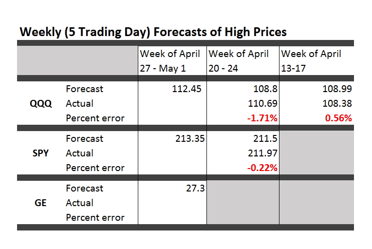
Here are forecasts of the weekly high price for three securities. These include intensely traded exchange traded funds (ETF’s) and a blue chip stock – QQQ, SPY, and GE.

The table also shows the track record so far.

All the numbers not explicitly indicated as percents are in US dollars.

These forecasts come with disclaimers. They are presented purely for scientific and informational purposes. This blog takes no responsibility for any investment gains or losses that might be linked with these forecasts. Invest at your own risk.

So having said that, some implications and background information.

First of all, it looks like it’s off to the races for the market as a whole this week, although possibly not for GE. The highs for the ETF’s all show solid gains.

Note, too, that these are forecasts of the high price which will be reached over the next five trading days, Monday through Friday of this week.

Key features of the method are now available in a white paper published under the auspices of the University of Munich – Predictability of the daily high and low of the S&P 500 index. This research shows that the so-called proximity variables achieve higher accuracies in predicting the daily high and low prices for the S&P 500 than do benchmark approaches, such as the no-change forecast and forecasts from an autoregressive model.

Again, caution is advised in making direct application of the methods in the white paper to the current problem –forecasting the high for a five day trading period. There have been many modifications.

That’s, of course, one reason for the public announcements of forecasts from the NPV (new proximity variable) model.

Go real-time, I’ve been advised. It makes the best case, or at least exposes the results to the light of day.

Based on backtesting, I expect forecasts for GE to be less accurate than those for QQQ and SPY. In terms of mean absolute percent error (MAPE), we are talking around 1% for QQQ and SPY and, maybe, 1.7% for GE.

The most reliable element of these forecasts are the indicated directions of change from the previous period highs.

Features and Implications

There are other several other features which are reliably predicted by the NPV models. For example, forecasts for the low price or even closing prices on Friday can be added – although closing prices are less reliable. Obviously, too, volatility metrics are implied by predictions of the high and low prices.

These five-trading day forecasts parallel the results for daily periods documented in the above-cited white paper. That is, the NPV forecast accuracy for these securities in each case beats “no-change” and autoregressive model forecasts.

Focusing on stock market forecasts has “kept me out of trouble” recently. I’m focused on quantitative modeling, and am not paying a lot of attention to global developments – such as the ever- impending Greek default or, possibly, exit from the euro. Other juicy topics include signs of slowing in the global economy, and the impact of armed conflict on the Arabian Peninsula on the global price of oil. These are great topics, but beyond hearsay or personal critique, it is hard to pin things down just now.

So, indeed, I may miss some huge external event which tips this frothy stock market into reverse – but, at the same time, I assure you, once a turning point from some external disaster takes place, the NPV models should do a good job of predicting the extent and duration of such a decline.

On a more optimistic note, my research shows the horizons for which the NPV approach applies and does a better job than the benchmark models. I have, for example, produced backtests for quarterly SPY data, demonstrating continuing superiority of the NPV method.

My guess – and I would be interested in validating this – is that the NPV approach connects with dominant trader practice. Maybe stock market prices are, in some sense, a random walk. But the reactions of traders to daily price movements create short term order out of randomness. And this order can emerge and persist for relatively long periods. And, not only that, but the NPV approach is linked with self-reinforcing tendencies, so that awareness may just make predicted effects more pronounced. That is, if I tell you the high price of a security is going up over the coming period, your natural reaction is to buy in – thus reinforcing the prediction. And the prediction is not just public relations stunt or fluff. The first prediction is algorithmic, rather than wishful and manipulative. Thus, the direction of change is more predictable than the precise extent of price change.

In any case, we will see over coming weeks how well these models do.

financial risk management, stock trading algorithms, Uncategorized

Portfolio Analysis

March 30, 2015 Clive Jones

Greetings again. Took a deep dive into portfolio analysis for a colleague.

Portfolio analysis, of course, has been deeply influenced by Modern Portfolio Theory (MPT) and the work of Harry Markowitz and Robert Merton, to name a couple of the giants in this field.

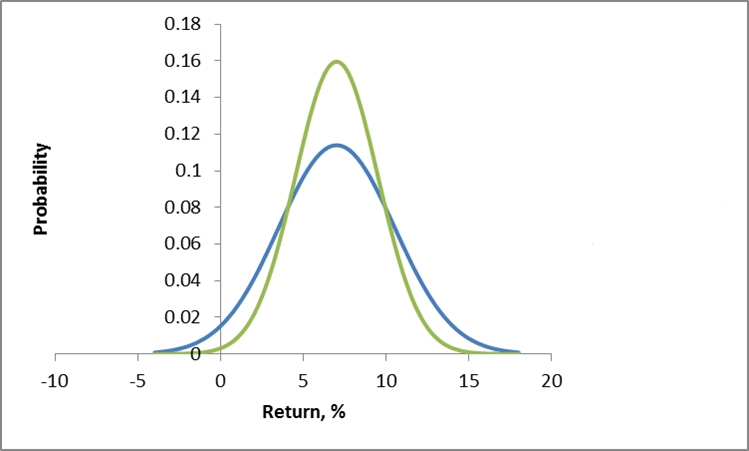
Conventionally, investment risk is associated with the standard deviation of returns. So one might visualize the dispersion of actual returns for investments around expected returns, as in the following chart.

Here, two investments have the same expected rate of return, but different standard deviations. Viewed in isolation, the green curve indicates the safer investment.

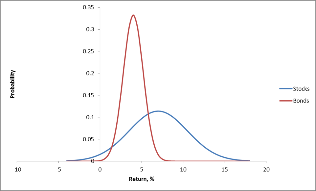
More directly relevant for portfolios are curves depicting the distribution of typical returns for stocks and bonds, which can be portrayed as follows.

Now the classic portfolio is comprised of 60 percent stocks and 40 percent bonds.

Where would its expected return be? Well, the expected value of a sum of random variables is the sum of their expected values. There is an algebra of expectations to express this around the operator E(.). So we have E(.6S+.4B)=.6E(S)+.4E(B), since a constant multiplied into a random variable just shifts the expectation by that factor. Here, of course, S stands for “stocks” and B “bonds.”

Thus, the expected return for the classic 60/40 portfolio is less than the returns that could be expected from stocks alone.

But the benefit here is that the risks have been reduced, too.

Thus, the variance of the 60/40 portfolio usually is less than the variance of a portfolio composed strictly of stocks.

One of the ways this is true is when the correlation or covariation of stocks and bonds is negative, as it has been in many periods over the last century. Thus, high interest rates mean slow to negative economic growth, but can be associated with high returns on bonds.

Analytically, this is because the variance of the sum of two random variables is the sum of their variances, plus their covariance multiplied by a factor of 2.

Thus, algebra and probability facts underpin arguments for investment diversification. Pick investments which are not perfectly correlated in their reaction to events, and your chances of avoiding poor returns and disastrous losses can be improved.

Implementing MPF

When there are more than two assets, you need computational help to implement MPT portfolio allocations.

For a general discussion of developing optimal portfolios and the efficient frontier see http://faculty.washington.edu/ezivot/econ424/portfoliotheorymatrixslides.pdf

There are associated R programs and a guide to using Excel’s Solver with this University of Washington course.

Also see Package ‘Portfolio’.

These programs help you identify the minimum variance portfolio, based on a group of assets and histories of their returns. Also, it is possible to find the minimum variance combination from a designated group of assets which meet a target rate of return, if, in fact, that is feasible with the assets in question. You also can trace out the efficient frontier – combinations of assets mapped in a space of returns and variances. These assets in each case have expected returns on the curve and are minimum variance compared with all other combinations that generate that rate of return (from your designated group of assets).

One of the governing ideas is that this efficient frontier is something an individual investor might travel along as they age – going from higher risk portfolios when they are younger, to more secure, lower risk portfolios, as they age.

Issues

As someone who believes you don’t really know something until you can compute it, it interests me that there are computational issues with implementing MPT.

I find, for example, that the allocations are quite sensitive to small changes in expected returns, variances, and the underlying covariances.

One of the more intelligent, recent discussions with suggested “fixes” can be found in An Improved Estimation to Make Markowitz’s Portfolio Optimization Theory Users Friendly and Estimation Accurate with Application on the US Stock Market Investment.

The more fundamental issue, however, is that MPT appears to assume that stock returns are normally distributed, when everyone after Mandelbrot should know this is hardly the case.

Again, there is a vast literature, but a useful approach seems to be outlined in Modelling in the spirit of Markowitz portfolio theory in a non-Gaussian world. These authors use MPT algorithms as the start of a search for portfolios which minimize value-at-risk, instead of variances.

Finally, if you want to cool off and still stay on point, check out the 2014 Annual Report of Berkshire Hathaway, and, especially, the Chairman’s Letter. That’s Warren Buffett who has truly mastered an old American form which I believe used to be called “cracker barrel philosophy.” Good stuff.

predictive analytics, stock market forecasts, time series forecasting

Trading Volume- Trends, Forecasts, Predictive Role

March 10, 2015 Clive Jones

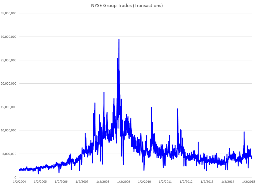
The New York Stock Exchange (NYSE) maintains a data library with historic numbers on trading volumes. Three charts built with some of this data tell an intriguing story about trends and predictability of volumes of transactions and dollars on the NYSE.

First, the number of daily transactions peaked during the financial troubles of 2008, only showing some resurgence lately.

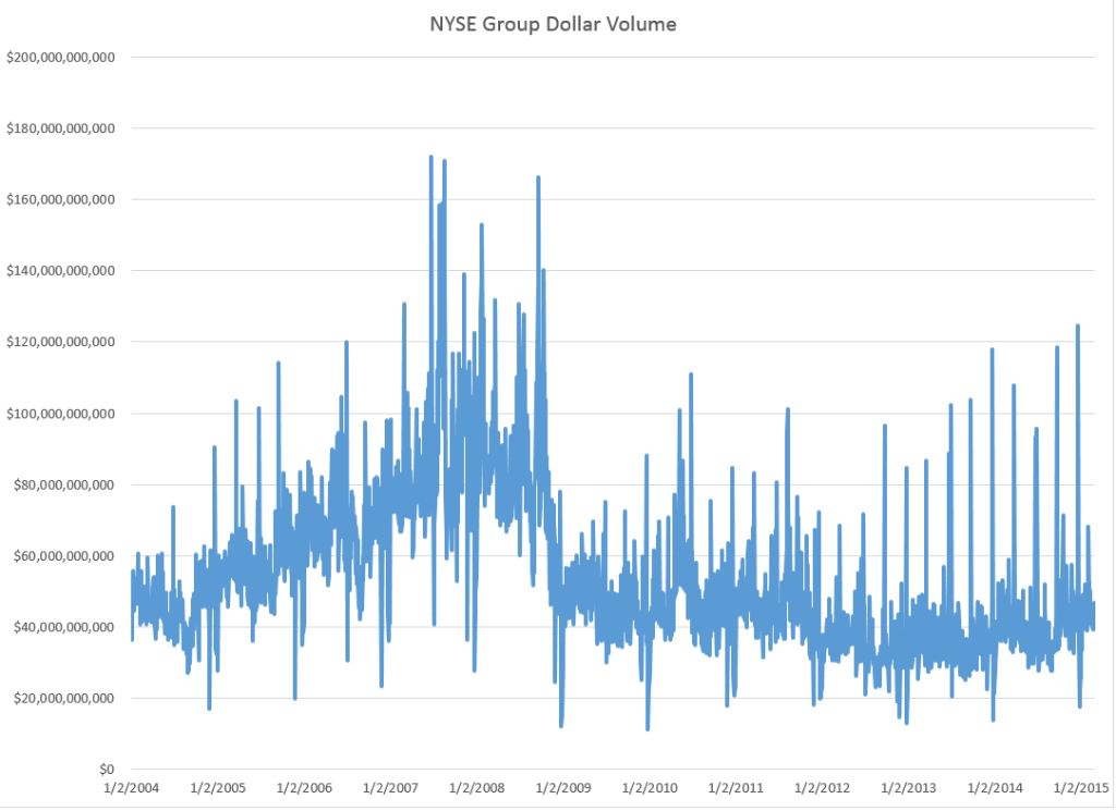
This falloff in the number of transactions is paralleled by the volume of dollars spent in these transactions.

These charts are instructive, since both highlight the existence of “spikes” in transaction and dollar volume that would seem to defy almost any run-of-the-mill forecasting algorithm. This is especially true for the transactions time series, since the spikes are more irregularly spaced. The dollar volume time series suggests some type of periodicity is possible for these spikes, particularly in recent years.

But lower trading volume has not impacted stock prices, which, as everyone knows, surged past 2008 levels some time ago.

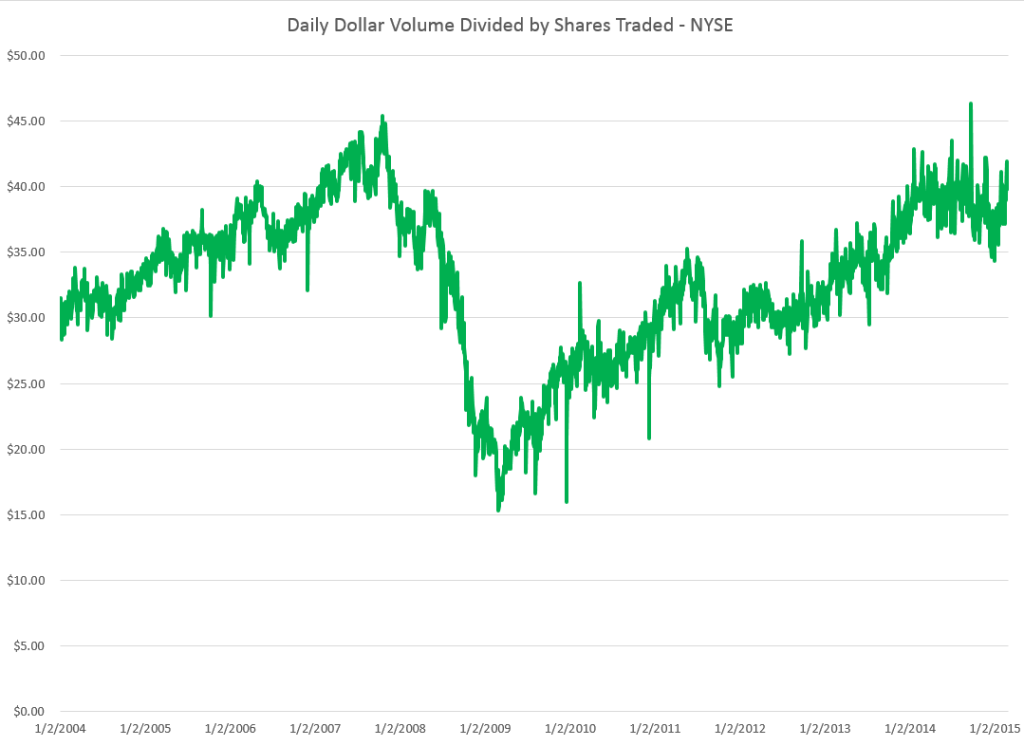
A raw ratio between the value of trades and NYSE stock transactions gives the average daily price per transaction.

So stock prices have rebounded, for the most part, to 2008 levels. Note here that the S&P 500 index stocks have done much better than this average for all stocks.

Why has trading volume declined on the NYSE? Some reasons gleaned from the commentariat.

Mom and Pop traders largely exited the market, after the crash of 2008
Some claim that program trading or high frequency trading peaked a few years back, and is currently in something of a decline in terms of its proportion of total stock transactions. This is, however, not confirmed by the NYSE Facts and Figures, which shows program trading pretty consistently at around 30 percent of total trading transactions..
Interest has shifted to options and futures, where trading volumes are rising.
Exchange Traded Funds (ETF’s) make up a larger portion of the market, and they, of course, do not actively trade.
Banks have reduced their speculation in equities, in anticipation of Federal regulations

See especially Market Watch and Barry Ritholtz on these trends.

But what about the impact of trading volume on price? That’s the real zinger of a question I hope to address in coming posts this week.

autoregressive model, machine learning, stock market forecasts, stock trading algorithms

The King Has No Clothes or Why There Is High Frequency Trading (HFT)

February 27, 2015 Clive Jones

I often present at confabs where there are engineers with management or executive portfolios. You start the slides, but, beforehand, prepare for the tough question. Make sure the numbers in the tables add up and that round-off errors or simple typos do not creep in to mess things up.

To carry this on a bit, I recall a Hewlett Packard VP whose preoccupation during meetings was to fiddle with their calculator – which dates the story a little. In any case, the only thing that really interested them was to point out mistakes in the arithmetic. The idea is apparently that if you cannot do addition, why should anyone believe your more complex claims?

I’m bending this around to the theory of efficient markets and rational expectations, by the way.

And I’m playing the role of the engineer.

Rational Expectations

The theory of rational expectations dates at least to the work of Muth in the 1960’s, and is coupled with “efficient markets.”

Lim and Brooks explain market efficiency in – The Evolution of Stock Market Efficiency Over Time: A Survey of the Empirical Literature

The term ‘market efficiency’, formalized in the seminal review of Fama (1970), is generally referred to as the informational efficiency of financial markets which emphasizes the role of information in setting prices.. More specifically, the efficient markets hypothesis (EMH) defines an efficient market as one in which new information is quickly and correctly reflected in its current security price… the weak-form version….asserts that security prices fully reflect all information contained in the past price history of the market.

Lim and Brooks focus, among other things, on statistical tests for random walks in financial time series, noting this type of research is giving way to approaches highlighting adaptive expectations.

Proof US Stock Markets Are Not Efficient (or Maybe That HFT Saves the Concept)

I like to read mathematically grounded research, so I have looked a lot of the papers purporting to show that the hypothesis that stock prices are random walks cannot be rejected statistically.

But really there is a simple constructive proof that this literature is almost certainly wrong.

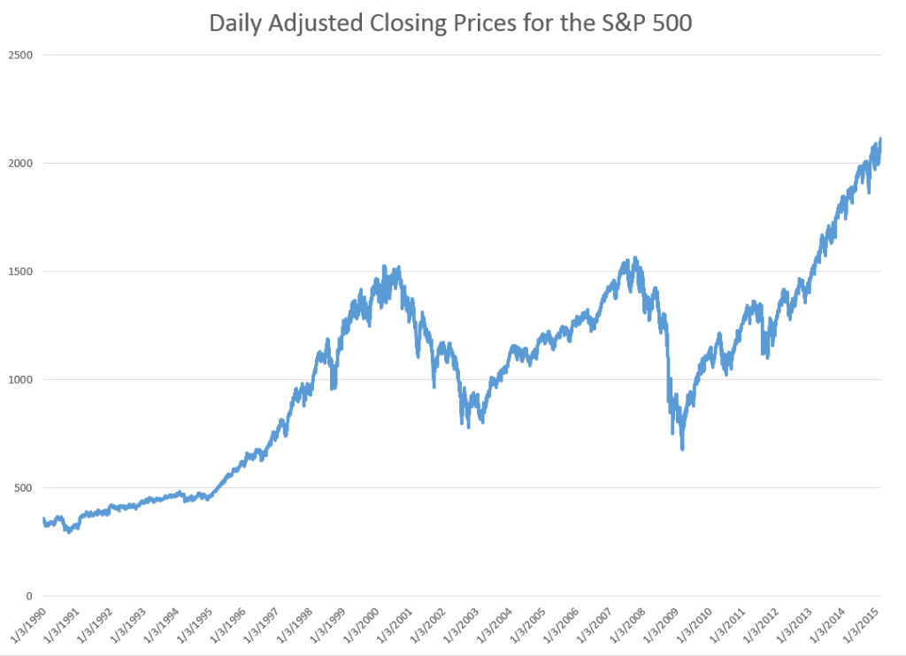
STEP 1: Grab the data. Download daily adjusted closing prices for the S&P 500 from some free site (e,g, Yahoo Finance). I did this again recently, collecting data back to 1990. Adjusted closing prices, of course, are based on closing prices for the trading day, adjusted for dividends and stock splits. Oh yeah, you may have to resort the data from oldest to newest, since a lot of sites present the newest data on top, originally.

Here’s a graph of the data, which should be very familiar by now.

STEP 2: Create the relevant data structure. In the same spreadsheet, compute the trading-day-over-treading day growth in the adjusted closing price (ACP). Then, side-by-side with this growth rate of the ACP, create another series which, except for the first value, maps the growth in ACP for the previous trading day onto the growth of the ACP for any particular day. That gives you two columns of new data.

STEP 3: Run adaptive regressions. Most spreadsheet programs include an ordinary least squares (OLS) regression routine. Certainly, Excel does. In any case, you want to setup up a regression to predict the growth in the ACP, based on one trading lags in the growth of the ACP.

I did this, initially, to predict the growth in ACP for January 3, 2000, based on data extending back to January 3, 1990 – a total of 2528 trading days. Then, I estimated regressions going down for later dates with the same size time window of 2528 trading days.

The resulting “predictions” for the growth in ACP are out-of-sample, in the sense that each prediction stands outside the sample of historic data used to develop the regression parameters used to forecast it.

It needs to be said that these predictions for the growth of the adjusted closing price (ACP) are marginal, correctly predicting the sign of the ACP only about 53 percent of the time.

An interesting question, though, is whether these just barely predictive forecasts can be deployed in a successful trading model. Would a trading algorithm based on this autoregressive relationship beat the proverbial “buy-and-hold?”

So, for example, suppose we imagine that we can trade at closing each trading day, close enough to the actual closing prices.

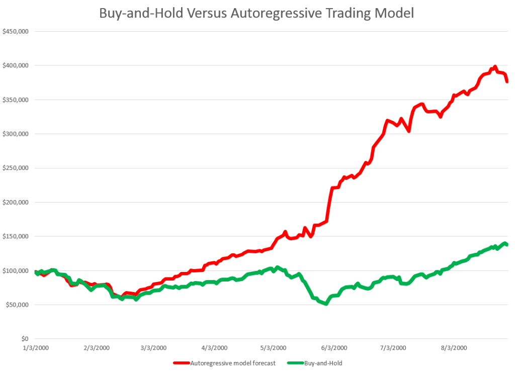
Then, you get something like this, if you invest $100,000 at the beginning of 2000, and trade through last week. If the predicted growth in the ACP is positive, you buy at the previous day’s close. If not, you sell at the previous day’s close. For the Buy-and-Hold portfolio, you just invest the $100,000 January 3, 2000, and travel to Tahiti for 15 years or so.

So, as should be no surprise, the Buy-and-Hold strategy results in replicating the S&P 500 Index on a $100,000 base.

The trading strategy based on the simple first order autoregressive model, on the other hand, achieves more than twice these cumulative earnings.

Now I suppose you could say that all this was an accident, or that it was purely a matter of chance, distributed over more than 3,810 trading days. But I doubt it. After all, this trading interval 2000-2015 includes the worst economic crisis since before World War II.

Or you might claim that the profits from the simple AR trading strategy would be eaten up by transactions fees and taxes. On this point, there were 1,774 trades, for an average of $163 per trade. So, worst case, if trading costs $10 a transaction, and there is a tax rate of 40 percent, that leaves $156K over these 14-15 years in terms of take-away profit, or about $10,000 a year.

Where This May Go Wrong

This does sound like a paen to stock market investing – even “day-trading.”

What could go wrong?

Well, I assume here, of course, that exchange traded funds (ETF’s) tracking the S&P 500 can be bought and sold with the same tactics, as outlined here.

Beyond that, I don’t have access to the data currently (although I will soon), but I suspect high frequency trading (HFT) may stand in the way of realizing this marvelous investing strategy.

So remember you have to trade some small instant before market closing to implement this trading strategy. But that means you get into the turf of the high frequency traders. And, as previous posts here observe, all kinds of unusual things can happen in a blink of an eye, faster than any human response time.

So – a conjecture. I think that the choicest situations from the standpoint of this more or less macro interday perspective, may be precisely the places where you see huge spikes in the volume of HFT. This is a proposition that can be tested.

I also think something like this has to be appealed to in order to save the efficient markets hypothesis, or rational expectations. But in this case, it is not the rational expectations of human subjects, but the presumed rationality of algorithms and robots, as it were, which may be driving the market, when push comes to shove.

Top picture from CommSmart Global.

European economy, financial forecasts, macroeconomic forecasting

The Greek Conundrum

February 17, 2015 Clive Jones

I’ve been focused on stock price forecast models, recently, and before that, on dynamics of oil prices.

However, it’s clear that almost any global market these days can be affected by developments in Europe.

There’s an excellent backgrounder to the crisis over restructuring Greek debt. See Greece, Its International Competitors and the Euro by the Turkish financial analyst T. Sabri Öncü – a PDF from the Economic and Political Weekly, an Indian Journal.

According to Öncü, the Greeks got in trouble with loans to finance consumption and nonproductive spending, when and after they joined the Eurozone in 2001. The extent of the problem was masked by accounting smoke and mirrors, only being revealed in 2009. Since then “bailouts” from European banking authorities have been designed to insure steady repayment of this debt to German and French banks, among others, although some Greek financial parties have benefited also.

Still, as Öncü writes,

Fast forward to today, despite two bailouts and adjustment programmes Greece has been in depression since the beginning of 2009. The Greece’s GDP is down about 25% from its peak in 2008, unemployment is at about 25%, youth unemployment is above 50%, Greece’s public debt to GDP ratio is at about a mind-boggling 175% and many Greeks are lining up for soup in front of soup kitchens reminiscent of the soup kitchens of the Great Depression of 1929.

As this post is written, negotiations between the new Syrizia government and European authorities have broken down, but here is an interesting video outlining the opposing positions, to an extent, prior to Monday.

Bruegel’s Interview: Debt Restructuring & Greece

Austerity is on the line here, since it seems clear Greece can never repay its debts as currently scheduled, even with imposing further privations on the Greek population.

self-fulfilling predictions, stock market forecasts

On Self-Fulfilling Prophecy

February 11, 2015 Clive Jones

In their excellent “Forecasting Stock Returns” in the Handbook of Economic Forecasting, David Rapach and Guofu Zhou write,

While stock return forecasting is fascinating, it can also be frustrating. Stock returns inherently contain a sizable unpredictable component, so that the best forecasting models can explain only a relatively small part of stock returns. Furthermore, competition among traders implies that once successful forecasting models are discovered, they will be readily adopted by others; the widespread adoption of successful forecasting models can then cause stock prices to move in a manner that eliminates the models’ forecasting ability..

Almost an article of faith currently, this perspective seems to rule out other reactions to forecasts which have been important in economic affairs, namely the self-fulfilling prophecy.

Now as “self-fulfilling prophecy” entered the lexicon, it was a prediction which originally was in error, but it became true, because people believed it was true and acted upon it.

Bank runs are the classic example.

The late Robert Merton wrote of the Last National Bank in his classic Social Theory and Social Structure, but there is no need for recourse to apocryphal history. Gary Richardson of the Federal Reserve Bank of Richmond has a nice writeup – Banking Panics of 1930 and 1931 –

..Caldwell was a rapidly expanding conglomerate and the largest financial holding company in the South. It provided its clients with an array of services – banking, brokerage, insurance – through an expanding chain controlled by its parent corporation headquartered in Nashville, Tennessee. The parent got into trouble when its leaders invested too heavily in securities markets and lost substantial sums when stock prices declined. In order to cover their own losses, the leaders drained cash from the corporations that they controlled.

On November 7, one of Caldwell’s principal subsidiaries, the Bank of Tennessee (Nashville) closed its doors. On November 12 and 17, Caldwell affiliates in Knoxville, Tennessee, and Louisville, Kentucky, also failed. The failures of these institutions triggered a correspondent cascade that forced scores of commercial banks to suspend operations. In communities where these banks closed, depositors panicked and withdrew funds en masse from other banks. Panic spread from town to town. Within a few weeks, hundreds of banks suspended operations. About one-third of these organizations reopened within a few months, but the majority were liquidated (Richardson 2007).

Of course, most of us know but choose to forget these examples, for a variety of reasons – the creation of the Federal Deposit Insurance Corporation has removed most of the threat, that was a long time ago, and so forth.

So it was with interest that I discovered a recent paper of researchers at Cal Tech and UCLA’s Andersson Management School The Self Fulfilling Prophecy of Popular Asset Pricing Models. The authors explore the impact of delegating investment decisions to investment professionals who, by all evidence, apply discounted cash flow models that are disconnected from investor’s individual utility functions.

Despite its elegance, the consumption-based model has one glaring deficiency.

The standard model and its more conventional variants have failed miserably at explaining the cross-section of returns; even tortured versions of the standard model have struggled to match data.

The authors then propose a Gendanken experiment where discounted cash flow models are used by the professional money managers who are delegated to invest by individuals.

The upshot –

Our thought experiment has an intriguing and heretofore unappreciated implication— there is a feedback relation between asset pricing models and the cross-section of expected returns. Our analysis implies that the cross-section of expected returns is not only described by theories of asset pricing, it is also determined by them.

I think Cornell and Hsu are on to something here.

More specifically, I have been trying to understand how to model a trading situation in which predictions of stock high and low prices in a period are self-confirming or self-fulfilling.

Suppose my prediction is that the daily high of Dazzle will be above yesterday’s daily high, if the opening price is above yesterday’s opening price. Then, if this persuades you to buy shares of Dazzle, it would seem that you contribute to the tendency for the stock price to increase. Furthermore, I don’t tell you exactly when the daily high will be reached, so I sort of put you in play. The onus is on you to make the right moves. The forecast does not come under suspicion.

As something of a data scientist, I think I can report that models of stock market trading at the level of agents participating in the market are not a major preoccupation of market analysts or theorists. The starting point seems to be Walras and the problem is how to set the price adjustment mechanism, since the tatonnement is obviously unrealistic

That then brings us probably to experimental economics, which shares a lot of turf with what is called behavioral economics.

The other possibility is simply to observe stock market prices and show that, quite generally, this type of rule must be at play and, because it is not inherently given to be true, it furthermore must be creating the conditions of its own success, to an extent.

financial forecasting, stock market forecasts, stock trading algorithms

Predicting the High of SPY Over Daily, Weekly, and Monthly Forecast Horizons

January 16, 2015 Clive Jones

Here are some remarkable findings relating to predicting the high and low prices of the SPDR S&P 500 ETF (SPY) in daily, weekly, and monthly periods.

Basically, the high and low prices for SPY can be forecast with some accuracy – especially with regards the sign of the percent change from the high or low of the previous period.

The simplicity of the predictive relationships are remarkable, and key off the ratio of the previous period high or low to the opening price for the new period under consideration. There is precedent in the work of George and Hwang, for example, who show picking portfolios of stocks whose price is near their 52-week high can generate superior returns (validated in 2010 for international portfolios). But my analysis concerns a specific exchange traded fund (ETF) which, of course, mirrors the S&P 500 Index.

Evidence

For data, I utilize daily, weekly, and monthly open, close, high, low, and volume data on the SPDR S&P 500 ETF SPY from Yahoo Finance from January 1993 to the present.

I estimate ordinary least squares (OLS) regression estimates on a rolling or adaptive basis.

So, for example, I begin weekly estimates to predict the high for a forecast horizon of one week on the period February 1, 1993 to December 12, 1994. The dependent variable is the growth in the highs from week to week – 97 observations on weekly data to begin with.

The initial regression has a coefficient of determination of 0.405 and indicates high statistical significance for the regression coefficients – although the underlying stochastic elements here are probably profoundly non-normal.

I use a similar setup to predict the weekly low of SPY, substituting the “growth” of the preceding low (in the previous week) to the current opening price in the set of explanatory variables. I continue using the lagged logarithm of the trading volume.

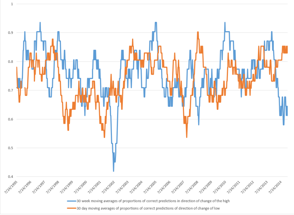
This chart shows the proportion of correct signs predicted by weekly models for the growth or percentage changes in the high and low prices in terms of 30 week moving averages (click to enlarge).

There is a lot to think about in this chart, clearly.

The basic truth, however, is that the predictive models, which are simple OLS regressions with two explanatory variables, predict the correct sign of the growth weekly percentage changes in the high and low SPY prices about 75 percent of the time.

Similar analysis of monthly data also leads to predictive models for the monthly high and lows. The predictive models for the high and low prices in monthly forecast horizons correctly predict more than 70 percent of the directions of change in these respective growth rates, with the model for the lows being more powerful statistically.

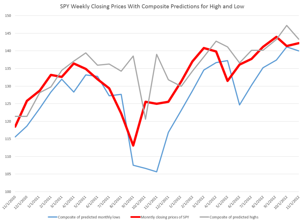
The actual forecasts of the growth in the monthly highs and lows may be helpful in discerning turning points in the SPY and, thus, the S&P 500, as the following chart suggests.

Here I apply the predicted high and low growth rates week-by-week to the previous week values for the high and low and also chart the SPY closing prices for the week (in bold red).

For discussion of the models for the daily highs and lows, see my previous blog posts here and here.

I might add that these findings relating to predicatability of the high and low of SPY on a daily, weekly, and monthly basis are among the strongest and simplest statistical relationships I have had the fortune to encounter.

Academic researchers are free to use and build on these results, but I would appreciate being credited with the underlying insight or as at least a source.

Discussion – Pathways of Predictability

Since this is not a refereed publication, I take the liberty of offering some conjectures on why this predictability exists.

My basic idea is that there are positive feedback loops for investing, based on fairly simple predictive models for the high of SPY that will be reached over a day, a week, or a month. So this would mean investors are aware of this relationship, and act upon it in real time. Their actions, furthermore, reinforce the strength of the relationship, creating pathways of predictability into the future in otherwise highly volatile, noisy data. Discovery of such pathways serves to reinforce their existence.

If this is true, it is real news and something relatively novel in economic forecasting.

And there is a second conjecture. I suspect that these “pathways of predictability” in the high and probably the low of SPY give us a window into turning points in the underlying stock index, the S&P 500. It should be possible to array daily, weekly, and monthly forecasts of the highs and lows for SPY and get some indication of a change in the direction of movement of the series.

These are a big claims, and eventually, may become shaded in colors of lighter and darker grey. However, I believe they work well as research hypotheses.

bagging, stock market forecasts, stock trading algorithms, time series forecasting

Revisiting the Predictability of the S&P 500

January 10, 2015 Clive Jones

Almost exactly a year ago, I posted on an algorithm and associated trading model for the S&P 500, the stock index which supports the SPY exchange traded fund.

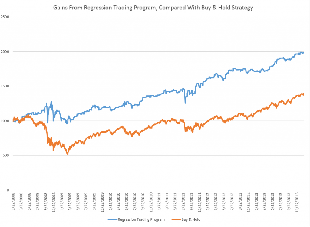
I wrote up an autoregressive (AR) model, using daily returns for the S&P 500 from 1993 to early 2008. This AR model outperforms a buy-and-hold strategy for the period 2008-2013, as the following chart shows.

The trading algorithm involves “buying the S&P 500” when the closing price indicates a positive return for the following trading day. Then, I “close out the investment” the next trading day at that day’s closing price. Otherwise, I stay in cash.

It’s important to be your own worst critic, and, along those lines, I’ve had the following thoughts.

First, the above graph disregards trading costs. Your broker would have to be pretty forgiving to execute 2000-3000 trades for less than the $500 you make over the buy-and-hold strategy. SO, I should deduct something for the trades in calculating the cumulative value.

The other criticism concerns high frequency trading. The daily returns are calculated against closing values, but, of course, to use this trading system you have to trade prior to closing. However, even a few seconds can make a crucial difference in the price of the S&P 500 or SPY – and even smaller intervals.

An Up-Dated AR Model

Taking some of these criticisms into account, I re-estimate an autoregressive model on more recent data –again calculating returns against closing prices on successive trading days.

This time I start with an initial investment of $100,000, and deduct $5 per trade off the totals as they cumulate.

I also utilize only seven (7) lags for the daily returns. This compares with the 30 lag model from the post a year ago, and I estimate the current model with OLS, rather than maximum likelihood.

The model is

R_t = 0.0007-0.0651R_t-1+0.0486R_t-2-0.0999R_t-3-0.0128R_t-4-0.1256R_t-5+0.0063R_t-6-0.0140R_t-7

where R_t is the daily return for trading day t. This model originates on data from June 11, 2011. The coefficients of the equation result from bagging OLS regressions – developing coefficient estimates for 100,000 similar size samples drawn with replacement from this dataset of 809 observations. These 100,000 coefficient estimates are averaged to arrive at the numbers shown above.

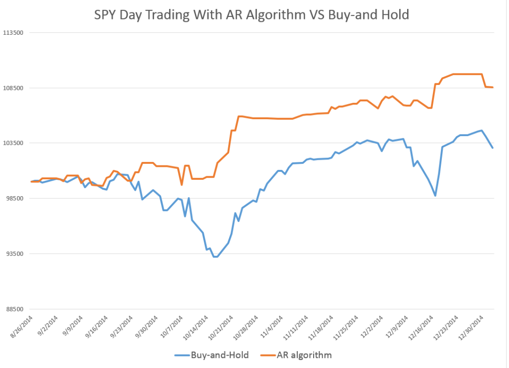
Here is the result of applying my revised model to recent stock market activity. The results are out-of-sample. In other words, I use the predictive equation which is calculated over data prior to the start of the investment comparison. I also filter the positive predictions for the next day closing price, only acting when they are a certain size or larger.

There is a 2-3 percent return on a hundred thousand dollar investment in one month, and a projected annual return on the order of 20-30 percent.

The current model also correctly predicts the sign of the daily return 58 percent of the time, compared with a much lower figure for the model from a year ago.

This looks like the best thing since sliced bread.

But wait – what about high frequency trading?

I’m exploring the implementation of this model – and maybe should never make it public.

But let me clue you in on what I suspect, and some evidence I have.

So, first, it is interesting the gains from trading on closing day prices more than evaporate by the opening of the New York Stock Exchange, following the generation of a “buy” signal according to this algorithm.

In other words, if you adjust the trading model to buy at the open of the following trading day, when the closing price indicates a positive return for the following day – you do not beat a buy-and-hold strategy. Something happens between the closing and the opening of the NYSE market for the SPY.

Someone else knows about this model?

I’m exploring the “final second’ volatility of the market, focusing on trading days when the closing prices look like they might come in to indicate a positive return the following day. This is complicated, and it puts me into issues of predictability in high frequency data.

I also am looking at the SPY numbers specifically to bring this discussion closer to trading reality.

Bottom line – It’s hard to make money in the market on trading algorithms if you are a day-trader – although probably easier with a super-computer at your command and when you sit within microseconds of executing an order on the NY Stock Exchange.

But these researches serve to indicate one thing fairly clearly. And that is that there definitely are aspects of stock prices which are predictable. Acting on the predictions is the hard part.

And Postscript: Readers may have noticed a lesser frequency of posting on Business Forecast blog in the past week or so. I am spending time running estimations and refreshing and extending my understanding of some newer techniques. Keep checking in – there is rapid development in “real world forecasting” – exciting and whiz bang stuff. I need to actually compute the algorithms to gain a good understanding – and that is proving time-consuming. There is cool stuff in the data warehouse though.

Big Data, business cycle, forecasting research, macroeconomic forecasting, predicting recessions

The Holy Grail of Business Forecasting – Forecasting the Next Downturn

September 29, 2014 Clive Jones

What if you could predict the Chicago Fed National Activity Index (CFNAI), interpolated monthly values of the growth of nominal GDP, the Aruoba-Diebold-Scotti (ADS) Business Conditions Index, and the Kansas City Financial Stress Index (KCFSI) three, five, seven, even twelve months into the future? What if your model also predicted turning points in these US indexes, and also similar macroeconomic variables for countries in Asia and the European Union? And what if you could do all this with data on monthly returns on the stock prices of companies in the financial sector?

That’s the claim of Linda Allen, Turan Bali, and Yi Tang in a fascinating 2012 paper Does Systemic Risk in the Financial Sector Predict Future Economic Downturns?

I’m going to refer to these authors as Bali et al, since it appears that Turan Bali, shown below, did some of the ground-breaking research on estimating parametric distributions of extreme losses. Bali also is the corresponding author.

Bali et al develop a new macroindex of systemic risk that predicts future real economic downturns which they call CATFIN.

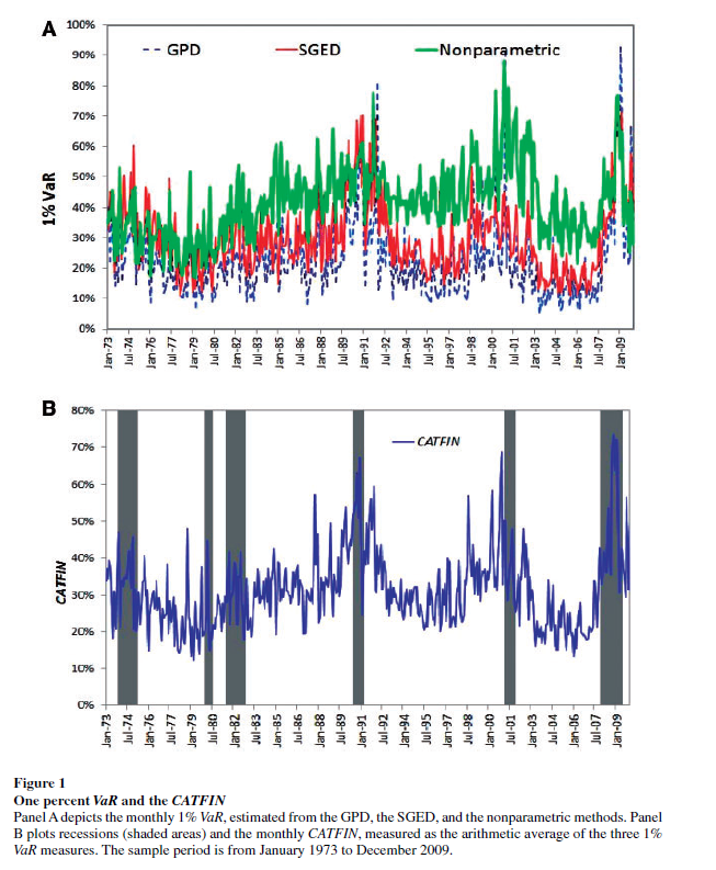
CATFIN is estimated using both value-at-risk (VaR) and expected shortfall (ES) methodologies, each of which are estimated using three approaches: one nonparametric and two different parametric specifications. All data used to construct the CATFIN measure are available at each point in time (monthly, in our analysis), and we utilize an out-of-sample forecasting methodology. We find that all versions of CATFIN are predictive of future real economic downturns as measured by gross domestic product (GDP), industrial production, the unemployment rate, and an index of eighty-five existing monthly economic indicators (the Chicago Fed National Activity Index, CFNAI), as well as other measures of real macroeconomic activity (e.g., NBER recession periods and the Aruoba-Diebold-Scott [ADS] business conditions index maintained by the Philadelphia Fed). Consistent with an extensive body of literature linking the real and financial sectors of the economy, we find that CATFIN forecasts aggregate bank lending activity.

The following graphic illustrates three components of CATFIN and the simple arithmetic average, compared with US recession periods.

Thoughts on the Method

OK, here’s the simple explanation. First, these researchers identify US financial companies based on definitions in Kenneth French’s site at the Tuck School of Business (Dartmouth). There are apparently 500-1000 of these companies for the period 1973-2009. Then, for each month in this period, rates of return of the stock prices of these companies are calculated. Then, three methods are used to estimate 1% value at risk (VaR) – two parametric methods and one nonparametric methods. The nonparametric method is straight-forward –

The nonparametric approach to estimating VaR is based on analysis of the left tail of the empirical return distribution conducted without imposing any restrictions on the moments of the underlying density…. Assuming that we have 900 financial firms in month t , the nonparametric measure of1%VaR is the ninth lowest observation in the cross-section of excess returns. For each month, we determine the one percentile of the cross-section of excess returns on financial firms and obtain an aggregate 1% VaR measure of the financial system for the period 1973–2009.

So far, so good. This gives us the data for the graphic shown above.

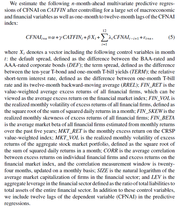
In order to make this predictive, the authors write that –

Like a lot of leading indicators, the CATFIN predictive setup “over-predicts” to some extent. Thus, there are there are five instances in which a spike in CATFIN is not followed by a recession, thereby providing a false positive signal of future real economic distress. However, the authors note that in many of these cases, predicted macroeconomic declines may have been averted by prompt policy intervention. Their discussion of this is very interesting, and plausible.

What This Means

The implications of this research are fairly profound – indicating, above all, the priority of the finance sector in leading the overall economy today. Certainly, this consistent with the balance sheet recession of 2008-2009, and probably will continue to be relevant going forward – since nothing really has changed and more concentration of ownership in finance has followed 2008-2009.

I do think that Serena Ng’s basic point in a recent review article probably is relevant – that not all recessions are the same. So it may be that this method would not work as well for, say, the period 1945-1970, before financialization of the US and global economies.

The incredibly ornate mathematics of modeling the tails of return distributions are relevant in this context, incidentally, since the nonparametric approach of looking at the empirical distributions month-by-month could be suspect because of “cherry-picking.” So some companies could be included, others excluded to make the numbers come out. This is much difficult in a complex maximum likelihood estimation process for the location parameters of these obscure distributions.

So the question on everybody’s mind is – WHAT DOES THE CATFIN MODEL INDICATE NOW ABOUT THE NEXT FEW MONTHS? Unfortunately, I am unable to answer that, although I have corresponded with some of the authors to inquire whether any research along such lines can be cited.

Bottom line – very impressive research and another example of how important science can get lost in the dance of prestige and names.

autoregressive model, volatility forecasting

Video Friday – Volatility

September 26, 2014 Clive Jones

Here are a couple of short YouTube videos from Bionic Turtle on estimating a GARCH (generalized autoregressive conditional heteroskedasticity) model and the simpler exponentially weighted moving average (EWMA) model.

GARCH models are designed to capture the clustering of volatility illustrated in the preceding post.

Forecast volatility with GARCH(1,1)

The point is that the parameters of a GARCH model are estimated over historic data, so the model can be utilized prospectively, to forecast future volatility, usually in the near term.

EWMA models, insofar as they put more weight on recent values, than on values more distant back in time, also tend to capture clustering phenomena.

Here is a comparison.

EWMA versus GARCH(1,1) volatility

Several of the Bionic Turtle series on estimating financial metrics are worth checking out.

Business Forecasting