Category Archives: causal discovery

Reading the Tea Leaves – Forecasts of Stock High and Low Prices

The residuals of predictive models are central to their statistical evaluation – with implications for confidence intervals of forecasts.

Of course, another name for the residuals of a predictive model is their errors.

Today, I want to present some information on the errors for the forecast models that underpin the Monday morning forecasts in this blog.

The results are both reassuring and challenging.

The good news is that the best fit distributions support confidence intervals, and, in some cases, can be viewed as transformations of normal variates. This is by no means given, as monstrous forms such as the Cauchy distribution sometimes present themselves in financial modeling as a best candidate fit.

The challenge is that the skew patterns of the forecasts of the high and low prices are weirdly symmetric. It looks to me as if traders tend to pile on when the price signals are positive for the high, or flee the sinking ship when the price history indicates the low is going lower.

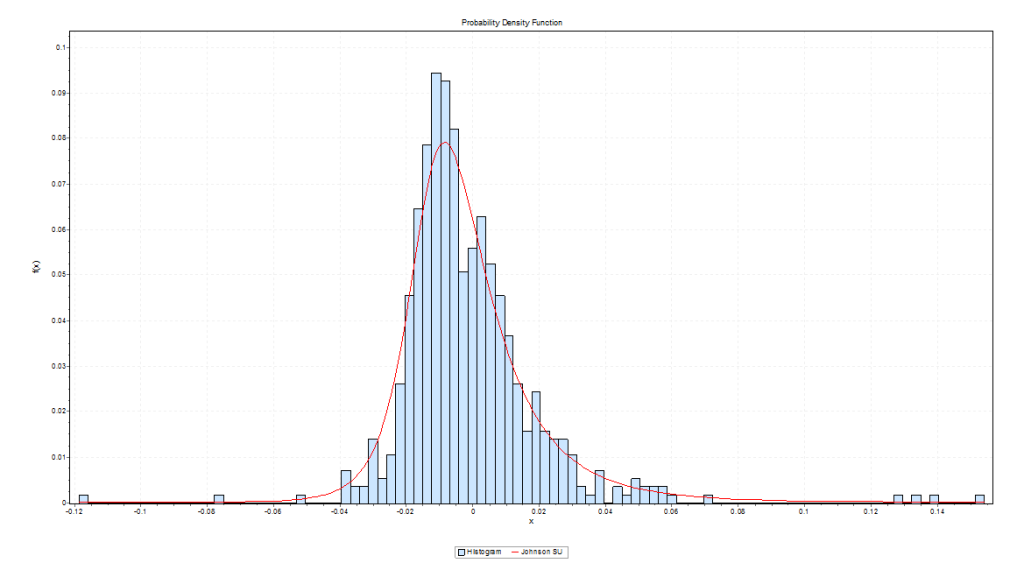
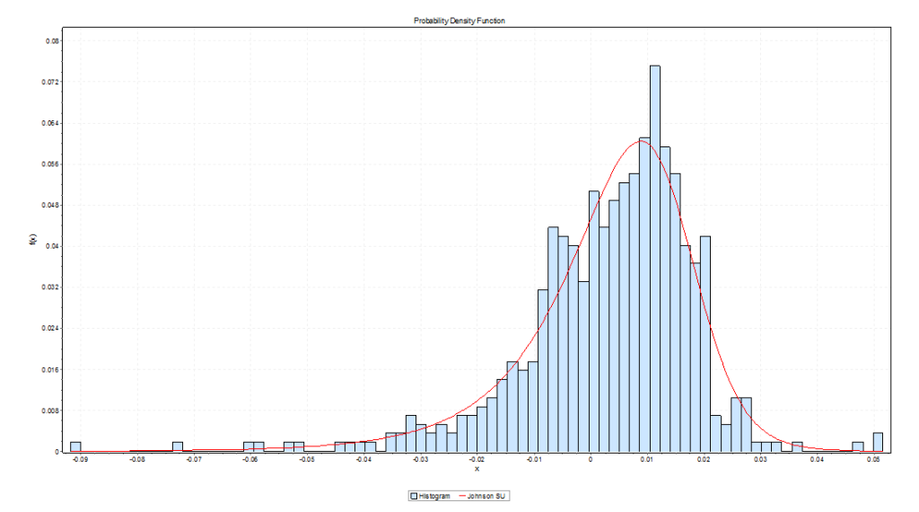
Here is the error distribution of percent errors for backtests of the five day forecast of the QQQ high, based on an out-of-sample study from 2004 to the present, a total of 573 five consecutive trading day periods.

JohnSUHigh

Here is the error distribution of percent errors for backtests of the five day forecast of the QQQ low.

JohnSULow

In the first chart for forecasts of high prices, errors are concentrated in the positive side of the percent error or horizontal axis. In the second graph, errors from forecasts of low prices are concentrated on the negative side of the horizontal axis.

In terms of statistics-speak, the first chart is skewed to the left, having a long tail of values to the left, while the second chart is skewed to the right.

What does this mean? Well, one interpretation is that traders are overshooting the price signals indicating a positive change in the high price or a lower low price.

Thus, the percent error is calculated as

(Actual – Predicted)/Actual

So the distribution of errors for forecasts of the high has an average which is slightly greater than zero, and the average for errors for forecasts of the low is slightly negative. And you can see the bulk of observations being concentrated, on the one hand, to the right of zero and, on the other, to the left of zero.

I’d like to find some way to fill out this interpretation, since it supports the idea that forecasts in this context are self-reinforcing, rather than self-nihilating.

I have more evidence consistent with this interpretation. So, if traders dive in when prices point to a high going higher, predictions of the high should be more reliable vis a vis direction of change with bigger predicted increases in the high. That’s also verifiable with backtests.

I use MathWave’s EasyFit. It’s user-friendly, and ranks best fit distributions based on three standard metrics of goodness of fit – the Chi-Squared, Komogorov-Smirnov, and Anderson-Darling statistics. There is a trial download of the software, if you are interested.

The Johnson SU distribution ranks first for the error distribution for the high forecasts, in terms of EasyFit’s measures of goodness of fit. The Johnson SU distribution also ranks first for Chi-Squared and the Anderson-Darling statistics for the errors of forecasts of the low.

This is an interesting distribution which can be viewed as a transformation of normal variates and which has applications, apparently, in finance (See http://www.ntrand.com/johnson-su-distribution/).

It is something I have encountered repeatedly in analyzing errors of proximity variable models. I am beginning to think it provides the best answer in determining confidence intervals of the forecasts.

Top picture from mysteryarts


2014 in Review – I

I’ve been going over past posts, projecting forward my coming topics. I thought I would share some of the best and some of the topics I want to develop.

Recommendations From Early in 2014

I would recommend Forecasting in Data-Limited Situations – A New Day. There, I illustrate the power of bagging to “bring up” the influence of weakly significant predictors with a regression example. This is fairly profound. Weakly significant predictors need not be weak predictors in an absolute sense, providing you can bag the sample to hone in on their values.

There also are several posts on asset bubbles.

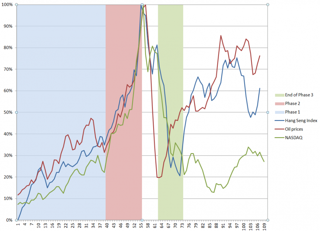
Asset Bubbles contains an intriguing chart which proposes a way to “standardize” asset bubbles, highlighting their different phases.

BubbleAnatomy

The data are from the Hong Kong Hang Seng Index, oil prices to refiners (combined), and the NASDAQ 100 Index. I arrange the series so their peak prices – the peak of the bubble – coincide, despite the fact that the peaks occurred at different times (October 2007, August 2008, March 2000, respectively). Including approximately 5 years of prior values of each time series, and scaling the vertical dimensions so the peaks equal 100 percent, suggesting three distinct phases. These might be called the ramp-up, faster-than-exponential growth, and faster-than-exponential decline. Clearly, I am influenced by Didier Sornette in choice of these names.

I’ve also posted several times on climate change, but I think, hands down, the most amazing single item is this clip from “Chasing Ice” showing calving of a Greenland glacier with shards of ice three times taller than the skyscrapers in Lower Manhattan.

See also Possibilities for Abrupt Climate Change.

I’ve been told that Forecasting and Data Analysis – Principal Component Regression is a helpful introduction. Principal component regression is one of the several ways one can approach the problem of “many predictors.”

In terms of slide presentations, the Business Insider presentation on the “Digital Future” is outstanding, commented on in The Future of Digital – I.

Threads I Want to Build On

There are threads from early in the year I want to follow up in Crime Prediction. Just how are these systems continuing to perform?

Another topic I want to build on is in Using Math to Cure Cancer. I’d like to find a sensitive discussion of how MD’s respond to predictive analytics sometime. It seems to me that US physicians are sometimes way behind the curve on what could be possible, if we could merge medical databases and bring some machine learning to bear on diagnosis and treatment.

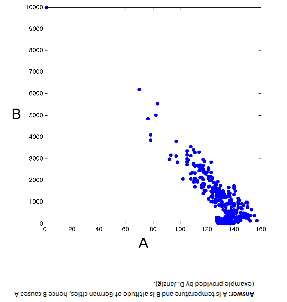
I am intrigued by the issues in Causal Discovery. You can get the idea from this chart. Here, B → A but A does not cause B – Why?

casualpic

I tried to write an informed post on power laws. The holy grail here is, as Xavier Gabaix says, robust, detail-independent economic laws.

Federal Reserve Policies

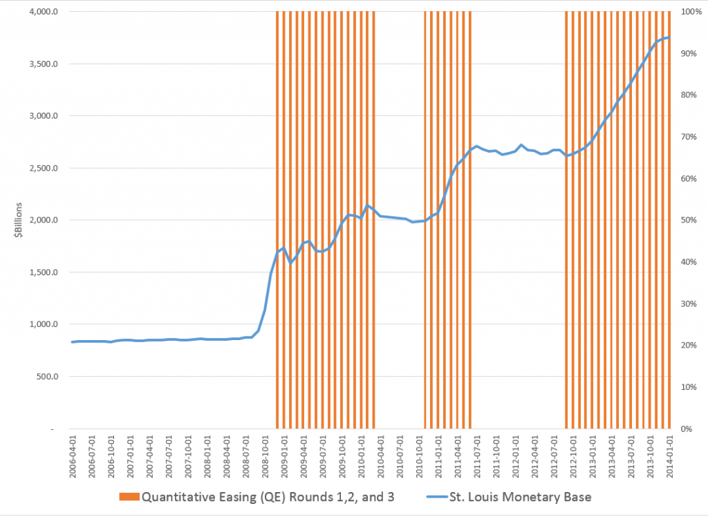
Federal Reserve policies are of vital importance to business forecasting. In the past two or three years, I’ve come to understand the Federal Reserve Balance sheet better, available from Treasury Department reports. What stands out is this chart, which anyone surfing finance articles on the net has seen time and again.

FedMBandQEgraph

This shows the total of the “monetary base” dating from the beginning of 2006. The red shaded areas of the graph indicate the time windows in which the various “Quantitative Easing” (QE) policies have been in effect – now three QE’s, QE1, QE2, and QE3.

Obviously, something is going on.

I had fun with this chart in a post called Rhino and Tapers in the Room – Janet Yellen’s Menagerie.

OK, folks, for this intermission, you might want to take a look at Malcolm Gladwell on the 10,000 Hour Rule


So what happens if you immerse yourself in all aspects of the forecasting field?

Coming – how posts in Business Forecast Blog pretty much establish that rational expectations is a concept way past its sell date.

Guy contemplating with wine at top from dreamstime.


Climate Change by 2030

Is climate change real? Is it predictable? How much warming can we expect by 2020 and then by 2030 in a business as usual scenario? How bad can it get? What about mitigation? Is there any credibility to the loud protestations of the climate change deniers? What about the so-called hockey stick and the exchange of sinister emails?

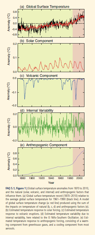
The Fifth Assessment Report of the Intergovernmental Panel on Climate Change (IPCC) addresses some of these questions. Its section The Physical Science Basis, which collates contributions of 250 scientists, contains this interesting graphic (click to enlarge) showing the upward trend in global temperature and the importance of the anthropogenic component, along with contributions from fluctuations in solar intensity and volcanic activity.

IPCCtemp

The Hockey Stick

Paleoclimate studies, also documented in this report, are the basis for the famous (notorious) hockey stick chart of long term global temperatures.

I was surprised to read, in catching up on this controversy, that the climate scientist Michael Mann who originated this chart has been totally vindicated (See The Hockey Stick: The Most Controversial Chart in Science, Explained).

Currently, scientific evidence suggests,

… present-day (2011) concentrations of the atmospheric greenhouse gases (GHGs) carbon dioxide (CO2), methane (CH4) and nitrous oxide (N2O) exceed the range of concentrations recorded in ice cores during the past 800,000 years. Past changes in atmospheric GHG concentrations can be determined with very high confidence1 from polar ice cores. Since AR4 these records have been extended from 650,000 years to 800,000 years ago.

The Drumbeat

In preparation for a September 23 summit, the UN has commissioned videos of weather forecasters supposedly announcing dire droughts, floods, and other weather catastrophes in 2050.

The IPCC also has videos. I include two – one on the physical science basis and the second on mitigation.

IPCC video 2013 –The Physical Science Basis

Climate summit 2014 – Mitigation

I personally am persuaded by the basic physics involved. As global GDP rises, so will energy consumption (although the details of this need to be examined carefully – conservation and change of technology can make big differences). In any case, more carbon dioxide and other similar gases will increase the greenhouse effect, raising global temperatures. It’s a good idea to call this climate change, rather than global warming, however, since volatility of weather patterns is a main result. There will be more climatic extremes, more droughts, but also more precipitation and flooding. Additionally, there could be changes in regional weather and climate patterns which could wreak havoc with the current distribution of population over geographic space. More rapid desertification is likely, and, of course, melting of glacial and polar ice will result in increases in sea level. And, as IPCC reports document, a lot of this is already happening.

There are, however, several problems that offer intellectual grounds for stalling the type of economic sacrifice that probably will be necessary to slow or reduce emissions.

First, there is the complexity of the evidence and argument, an issue flagged by Nate Silver recently. Secondly, there is the problem that, despite increases in greenhouse gas emissions after the turn of the century, there has been some leveling of global temperature increase, according to some metrics. Finally, there is the related problem of whether current climate models predict the recent past, whether they “retrodict.”

I’d like to address these issues or problems in a future post, along with my take on these projections or forecasts for 2020 and 2030.

LInks – late May

US and Global Economic Prospects

Goldman’s Hatzius: Rationale for Economic Acceleration Is Intact

We currently estimate that real GDP fell -0.7% (annualized) in the first quarter, versus a December consensus estimate of +2½%. On the face of it, this is a large disappointment. It raises the question whether 2014 will be yet another year when initially high hopes for growth are ultimately dashed.

 Today we therefore ask whether our forecast that 2014-2015 will show a meaningful pickup in growth relative to the first four years of the recovery is still on track. Our answer, broadly, is yes. Although the weak first quarter is likely to hold down real GDP for 2014 as a whole, the underlying trends in economic activity are still pointing to significant improvement….

 The basic rationale for our acceleration forecast of late 2013 was twofold—(1) an end to the fiscal drag that had weighed on growth so heavily in 2013 and (2) a positive impulse from the private sector following the completion of the balance sheet adjustments specifically among US households. Both of these points remain intact.

Economy and Housing Market Projected to Grow in 2015

Despite many beginning-of-the-year predictions about spring growth in the housing market falling flat, and despite a still chugging economy that changes its mind quarter-to-quarter, economists at the National Association of Realtors and other industry groups expect an uptick in the economy and housing market through next year.

The key to the NAR’s optimism, as expressed by the organization’s chief economist, Lawrence Yun, earlier this week, is a hefty pent-up demand for houses coupled with expectations of job growth—which itself has been more feeble than anticipated. “When you look at the jobs-to-population ratio, the current period is weaker than it was from the late 1990s through 2007,” Yun said. “This explains why Main Street America does not fully feel the recovery.”

Yun’s comments echo those in a report released Thursday by Fitch Ratings and Oxford Analytica that looks at the unusual pattern of recovery the U.S. is facing in the wake of its latest major recession. However, although the U.S. GDP and overall economy have occasionally fluctuated quarter-to-quarter these past few years, Yun said that there are no fresh signs of recession for Q2, which could grow about 3 percent.

Report: San Francisco has worse income inequality than Rwanda

If San Francisco was a country, it would rank as the 20th most unequal nation on Earth, according to the World Bank’s measurements.

Googlebus

Climate Change

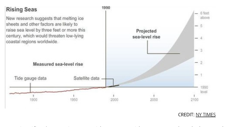
When Will Coastal Property Values Crash And Will Climate Science Deniers Be The Only Buyers?

sea

How Much Will It Cost to Solve Climate Change?

Switching from fossil fuels to low-carbon sources of energy will cost $44 trillion between now and 2050, according to a report released this week by the International Energy Agency.

Natural Gas and Fracking

How The Russia-China Gas Deal Hurts U.S. Liquid Natural Gas Industry

This could dampen the demand – and ultimately the price for – LNG from the United States. East Asia represents the most prized market for producers of LNG. That’s because it is home to the top three importers of LNG in the world: Japan, South Korea and China. Together, the three countries account for more than half of LNG demand worldwide. As a result, prices for LNG are as much as four to five times higher in Asia compared to what natural gas is sold for in the United States.

The Russia-China deal may change that.

If LNG prices in Asia come down from their recent highs, the most expensive LNG projects may no longer be profitable. That could force out several of the U.S. LNG projects waiting for U.S. Department of Energy approval. As of April, DOE had approved seven LNG terminals, but many more are waiting for permits.

LNG terminals in the United States will also not be the least expensive producers. The construction of several liquefaction facilities in Australia is way ahead of competitors in the U.S., and the country plans on nearly quadrupling its LNG capacity by 2017. More supplies and lower-than-expected demand from China could bring down prices over the next several years.

Write-down of two-thirds of US shale oil explodes fracking mythThis is big!

Next month, the US Energy Information Administration (EIA) will publish a new estimate of US shale deposits set to deal a death-blow to industry hype about a new golden era of US energy independence by fracking unconventional oil and gas.

EIA officials told the Los Angeles Times that previous estimates of recoverable oil in the Monterey shale reserves in California of about 15.4 billion barrels were vastly overstated. The revised estimate, they said, will slash this amount by 96% to a puny 600 million barrels of oil.

The Monterey formation, previously believed to contain more than double the amount of oil estimated at the Bakken shale in North Dakota, and five times larger than the Eagle Ford shale in South Texas, was slated to add up to 2.8 million jobs by 2020 and boost government tax revenues by $24.6 billion a year.

China

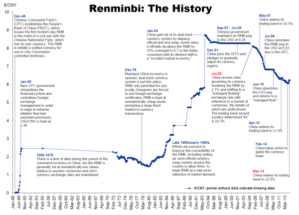
The Annotated History Of The World’s Next Reserve Currency

yuanhistory

Goldman: Prepare for Chinese property bust

…With demand poised to slow given a tepid economic backdrop, weaker household affordability, rising mortgage rates and developer cash flow weakness, we believe current construction capacity of the domestic property industry may be excessive. We estimate an inventory adjustment cycle of two years for developers, driving 10%-15% price cuts in most cities with 15% volume contraction from 2013 levels in 2014E-15E. We also expect M&A activities to take place actively, favoring developers with strong balance sheet and cash flow discipline.

China’s Shadow Banking Sector Valued At 80% of GDP

The China Banking Regulatory Commission has shed light on the country’s opaque shadow banking sector. It was as large as 33 trillion yuan ($5.29 trillion) in mid-2013 and equivalent to 80% of last year’s GDP, according to Yan Qingmin, a vice chairman of the commission.

In a Tuesday WeChat blog sent by the Chong Yang Institute for Financial Studies, Renmin University, Yan wrote that his calculation is based on shadow lending activities from asset management businesses to trust companies, a definition he said was very broad.  Yan said the rapid expansion of the sector, which was equivalent to 53% of GDP in 2012, entailed risks of some parts of the shadow banking business, but not necessarily the Chinese economy.

Yan’s estimation is notably higher than that of the Chinese Academy of Social Sciences. The government think tank said on May 9 that the sector has reached 27 trillion yuan ($4.4 trillion in 2013) and is equivalent to nearly one fifth of the domestic banking sector’s total assets.

Massive, Curvaceous Buildings Designed to Imitate a Mountain Forest

Chinamassive

Information Technology (IT)

I am an IT generalist. Am I doomed to low pay forever? Interesting comments and suggestions to this question on a Forum maintained by The Register.

I’m an IT generalist. I know a bit of everything – I can behave appropriately up to Cxx level both internally and with clients, and I’m happy to crawl under a desk to plug in network cables. I know a little bit about how nearly everything works – enough to fill in the gaps quickly: I didn’t know any C# a year ago, but 2 days into a project using it I could see the offshore guys were writing absolute rubbish. I can talk to DB folks about their DBs; network guys about their switches and wireless networks; programmers about their code and architects about their designs. Don’t get me wrong, I can do as well as talk, programming, design, architecture – but I would never claim to be the equal of a specialist (although some of the work I have seen from the soi-disant specialists makes me wonder whether I’m missing a trick).

My principle skill, if there is one – is problem resolution, from nitty gritty tech details (performance and functionality) to handling tricky internal politics to detoxify projects and get them moving again.

How on earth do I sell this to an employer as a full-timer or contractor? Am I doomed to a low income role whilst the specialists command the big day rates? Or should I give up on IT altogether

Crowdfunding is brutal… even when it works

China bans Windows 8

China has banned government use of Windows 8, Microsoft Corp’s latest operating system, a blow to a US technology company that has long struggled with sales in the country.

The Central Government Procurement Center issued the ban on installing Windows 8 on Chinese government computers as part of a notice on the use of energy-saving products, posted on its website last week.

Data Analytics

Statistics of election irregularities – good forensic data analytics.

Links – April 18

Ukraine

US financial showdown with Russia is more dangerous than it looks, for both sides Ambrose Evans-Pritchard at his most incisive.

How the Ukraine crisis ends Henry Kissinger, not always one of my favorites, writes an almost wise comment on the Ukraine from early March. Still relevant.

The West must understand that, to Russia, Ukraine can never be just a foreign country. Russian history began in what was called Kievan-Rus. The Russian religion spread from there. Ukraine has been part of Russia for centuries, and their histories were intertwined before then. Some of the most important battles for Russian freedom, starting with the Battle of Poltava in 1709 , were fought on Ukrainian soil. The Black Sea Fleet — Russia’s means of projecting power in the Mediterranean — is based by long-term lease in Sevastopol, in Crimea. Even such famed dissidents as Aleksandr Solzhenitsyn and Joseph Brodsky insisted that Ukraine was an integral part of Russian history and, indeed, of Russia.

China

The Future of Democracy in Hong Kong There is an enlightening video (about 1 hour long) interview with Veteran Hong Kong political leaders Anson Chan and Martin Lee. Beijing and local Hong Kong democratic rule appear to be on a collision course.

Inside Look At Electric Taxis Hitting China In Mass This Summer China needs these. The pollution in Beijing and other big cities from cars is stifling and getting worse.

taxi

Economy

Detecting bubbles in real time Interesting suggestion for metric to guage bubble status of an asset market.

Fed’s Yellen More Concerned About Inflation Running Below 2% Target Just a teaser, but check this Huffington Post flash video of Yellen, still at the time with the San Francisco Fed, as she lays out the dangers of deflation in early 2013. Note also the New Yorker blog on Yellen’s recent policy speech, and her silence on speculative bubbles.

Yellen

Data Analytics

Manipulate Me: The Booming Business in Behavioral Finance

Hidden Markov Models: The Backwards Algorithm

Suppose you are at a table at a casino and notice that things don’t look quite right. Either the casino is extremely lucky, or things should have averaged out more than they have. You view this as a pattern recognition problem and would like to understand the number of ‘loaded’ dice that the casino is using and how these dice are loaded. To accomplish this you set up a number of Hidden Markov Models, where the number of loaded die are the latent variables, and would like to determine which of these, if any, is more likely to be using rigged dice.

Tornado Frequency Distribution

Data analysis, data science, and advanced statistics have an important role to play in climate science.

James Elsner’s blog Hurricane & Tornado Climate offers salient examples, in this regard.

Yesterday’s post was motivated by an Elsner suggestion that the time trend in maximum wind speeds of larger or more powerful hurricanes is strongly positive since weather satellite observations provide better measurement (post-1977).

Here’s a powerful, short video illustrating the importance of proper data segmentation and statistical characterization for tornado data – especially for years of tremendous devastation, such as 2011.

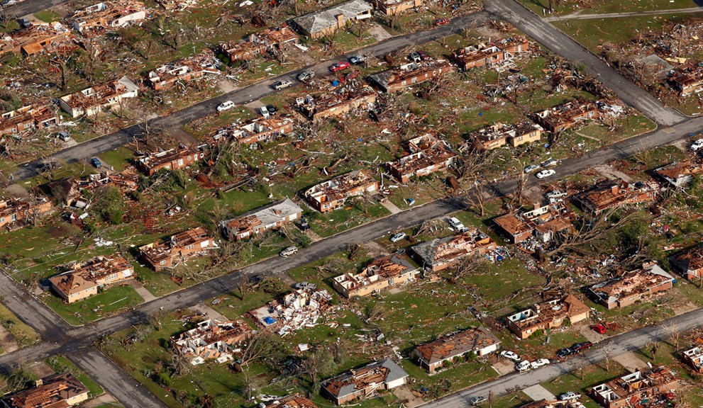
Events that year have a more than academic interest for me, incidentally, since my city of birth – Joplin, Missouri – suffered the effects of a immense supercell which touched down and destroyed everything in its path, including my childhood home. The path of this monster was, at points, nearly a mile wide, and it gouged out a track several miles through this medium size city.

Here is Elsner’s video integrating data analysis with matters of high human import.

There is a sort of extension, in my mind, of the rational expectations issue to impacts of climate change and extreme weather. The question is not exactly one people living in areas subject to these events might welcome. But it is highly relevant to data analysis and statistics.

The question simply is whether US property and other insurance companies are up-to-speed on the type of data segmentation and analysis that is needed to adequately capture the probable future impacts of some of these extreme weather events.

This may be where the rubber hits the road with respect to Bayesian techniques – popular with at least some prominent climate researchers, because they allow inclusion of earlier, less-well documented historical observations.

Quantile Regression

There’s a straight-forward way to understand the value and potential significance of quantile regression – consider the hurricane data referenced in James Elsner’s blog Hurricane & Tornado Climate.

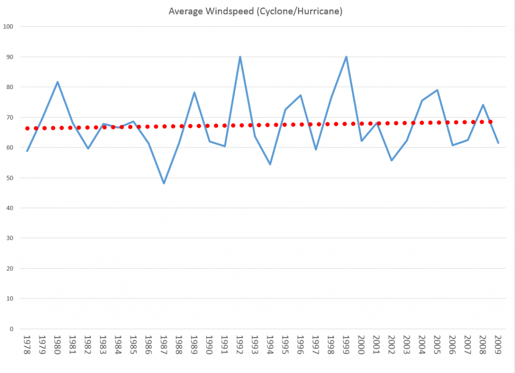
Here is a plot of average windspeed of hurricanes in the Atlantic and Gulf Coast since satellite observations began after 1977.

HurricaneAvgWS

Based on averages, the linear trend line increases about 2 miles per hour over this approximately 30 year period.

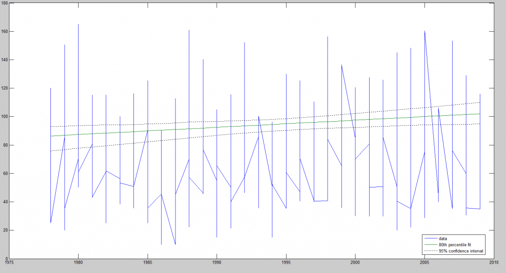
An 80th percentile quantile regression trend line, on the other hand, with this data indicates that the trend in the more violent hurricanes shows an about 15 mph increase over this same period.

HurricaneQuartileReg

In other words, if we look at the hurricanes which are in the 80th percentile or more, there is a much stronger trend in maximum wind speeds, than in the average for all US-related hurricanes in this period.

A quantile q, 0<q<1, splits the data into proportions q below and 1-q above. The most familiar quantile, thus, may be the 50th percentile which is the quantile which splits the data at the median – 50 percent below and 50 percent above.

Quantile regression (QR) was developed, in its modern incarnation by Koenker and Basset in 1978. QR is less influenced by non-normal errors and outliers, and provides a richer characterization of the data.

Thus, QR encourages considering the impact of a covariate on the entire distribution of y, not just is conditional mean.

Roger Koenker and Kevin F. Hallock’s Quantile Regression in the Journal of Economic Perspectives 2001 is a standard reference.

We say that a student scores at the tth quantile of a standardized exam if he performs better than the proportion t of the reference group of students and worse than the proportion (1–t). Thus, half of students perform better than the median student and half perform worse. Similarly, the quartiles divide the population into four segments with equal proportions of the reference population in each segment. The quintiles divide the population into five parts; the deciles into ten parts. The quantiles, or percentiles, or occasionally fractiles, refer to the general case.

Just as we can define the sample mean as the solution to the problem of minimizing a sum of squared residuals, we can define the median as the solution to the problem of minimizing a sum of absolute residuals.

Ordinary least squares (OLS) regression minimizes the sum of squared errors of observations minus estimates. This minimization leads to explicit equations for regression parameters, given standard assumptions.

Quantile regression, on the other hand, minimizes weighted sums of absolute deviations of observations on a quantile minus estimates. This minimization problem is solved by the simplex method of linear programming, rather than differential calculus. The solution is robust to departures from normality of the error process and outliers.

Koenker’s webpage is a valuable resource with directions for available software to estimate QR. I utilized Mathworks Matlab for my estimate of a QR with the hurricane data, along with a supplemental program for quantreg(.) I downloaded from their site.

Here are a couple of short, helpful videos from Econometrics Academy.

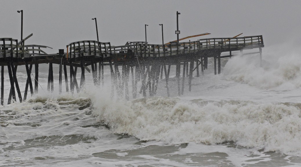
Featured image from http://www.huffingtonpost.com/2012/10/29/hurricane-sandy-apps-storm-tracker-weather-channel-red-cross_n_2039433.html

Possibilities for Abrupt Climate Change

The National Research Council (NRC) published ABRUPT IMPACTS OF CLIMATE CHANGE recently, downloadable from the National Academies Press website.

It’s the third NRC report to focus on abrupt climate change, the first being published in 2002. NRC members are drawn from the councils of the National Academy of Sciences, the National Academy of Engineering, and the Institute of Medicine.

The climate change issue is a profound problem in causal discovery and forecasting, to say the very least.

Before I highlight graphic and pictoral resources of the recent NRC report, let me note that Menzie Chin at Econbrowser posted recently on Economic Implications of Anthropogenic Climate Change and Extreme Weather. Chin focuses on the scientific consensus, presenting graphics illustrating the more or less relentless upward march of global average temperatures and estimates (by James Stock no less) of the man-made (anthropogenic) component.

The Econbrowser Comments section is usually interesting and revealing, and this time is no exception. Comments range from “climate change is a left-wing conspiracy” and arguments that “warmer would be better” to the more defensible thought that coming to grips with global climate change would probably mean restructuring our economic setup, its incentives, and so forth.

But I do think the main aspects of the climate change problem – is it real, what are its impacts, what can be done – are amenable to causal analysis at fairly deep levels.

To dispel ideological nonsense, current trends in energy use – growing globally at about 2 percent per annum over a long period – lead to the Earth becoming a small star within two thousand years, or less – generating the amount of energy radiated by the Sun. Of course, changes in energy use trends can be expected before then, when for example the average ambient temperature reaches the boiling point of water, and so forth. These types of calculations also can be made realistically about the proliferation of the automobile culture globally with respect to air pollution and, again, contributions to average temperature. Or one might simply consider the increase in the use of materials and energy for a global population of ten billion, up from today’s number of about 7 billion.

Highlights of the Recent NRC Report

It’s worth quoting the opening paragraph of the report summary –

Levels of carbon dioxide and other greenhouse gases in Earth’s atmosphere are exceeding levels recorded in the past millions of years, and thus climate is being forced beyond the range of the recent geological era. Lacking concerted action by the world’s nations, it is clear that the future climate will be warmer, sea levels will rise, global rainfall patterns will change, and ecosystems will be altered.

So because of growing CO2 (and other greenhouse gases), climate change is underway.

The question considered in ABRUPT IMPACTS OF CLIMATE CHANGE (AICH), however, is whether various thresholds will be crossed, whereby rapid, relatively discontinuous climate change occurs. Such abrupt changes – with radical shifts occurring over decades, rather than centuries – before. AICH thus cites,

..the end of the Younger Dryas, a period of cold climatic conditions and drought in the north that occurred about 12,000 years ago. Following a millennium-long cold period, the Younger Dryas abruptly terminated in a few decades or less and is associated with the extinction of 72 percent of the large-bodied mammals in North America.

The main abrupt climate change noted in AICH is rapid decline of the Artic sea ice. AICH puts up a chart which is one of the clearest examples of a trend you can pull from environmental science, I would think.
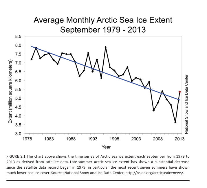
ArticSeaIce

AICH also puts species extinction front and center as a near-term and certain discontinuous effect of current trends.

Apart from melting of the Artic sea ice and species extinction, AICH lists destabilization of the Antarctic ice sheet as a nearer term possibility with dramatic consequences. Because a lot of this ice in the Antarctic is underwater, apparently, it is more at risk than, say, the Greenland ice sheet. Melting of either one (or both) of these ice sheets would raise sea levels tens of meters – an estimated 60 meters with melting of both.

Two other possibilities mentioned in previous NRC reports on abrupt climate change are discussed and evaluated as low probability developments until after 2100. These are stopping of the ocean currents that circulate water in the Atlantic, warming northern Europe, and release of methane from permafrost or deep ocean deposits.

The AMOC is the ocean circulation pattern that involves the northward flow of warm near-surface waters into the northern North Atlantic and Nordic Seas, and the south- ward flow at depth of the cold dense waters formed in those high latitude regions. This circulation pattern plays a critical role in the global transport of oceanic heat, salt, and carbon. Paleoclimate evidence of temperature and other changes recorded in North Atlantic Ocean sediments, Greenland ice cores and other archives suggest that the AMOC abruptly shut down and restarted in the past—possibly triggered by large pulses of glacial meltwater or gradual meltwater supplies crossing a threshold—raising questions about the potential for abrupt change in the future.

Despite these concerns, recent climate and Earth system model simulations indicate that the AMOC is currently stable in the face of likely perturbations, and that an abrupt change will not occur in this century. This is a robust result across many different models, and one that eases some of the concerns about future climate change.

With respect to the methane deposits in Siberia and elsewhere,

Large amounts of carbon are stored at high latitudes in potentially labile reservoirs such as permafrost soils and methane-containing ices called methane hydrate or clathrate, especially offshore in ocean marginal sediments. Owing to their sheer size, these carbon stocks have the potential to massively affect Earth’s climate should they somehow be released to the atmosphere. An abrupt release of methane is particularly worrisome because methane is many times more potent than carbon dioxide as a greenhouse gas over short time scales. Furthermore, methane is oxidized to carbon dioxide in the atmosphere, representing another carbon dioxide pathway from the biosphere to the atmosphere.

According to current scientific understanding, Arctic carbon stores are poised to play a significant amplifying role in the century-scale buildup of carbon dioxide and methane in the atmosphere, but are unlikely to do so abruptly, i.e., on a timescale of one or a few decades. Although comforting, this conclusion is based on immature science and sparse monitoring capabilities. Basic research is required to assess the long-term stability of currently frozen Arctic and sub-Arctic soil stocks, and of the possibility of increasing the release of methane gas bubbles from currently frozen marine and terrestrial sediments, as temperatures rise.

So some bad news and, I suppose, good news – more time to address what would certainly be completely catastrophic to the global economy and world population.

AICH has some neat graphics and pictoral exhibits.

For example, Miami Florida will be largely underwater within a few decades, according to many standard forecasts of increases in sea level (click to enlarge).
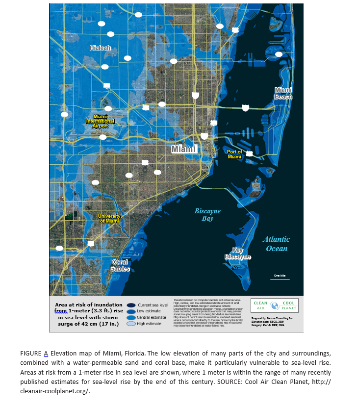
Florida

But perhaps most chilling of all (actually not a good metaphor here but you know what I mean) is a graphic I have not seen before, but which dovetails with my initial comments and observations of physicists.

This chart toward the end of the AICH report projects increase in global temperature beyond any past historic level (or prehistoric, for that matter) by the end of the century.
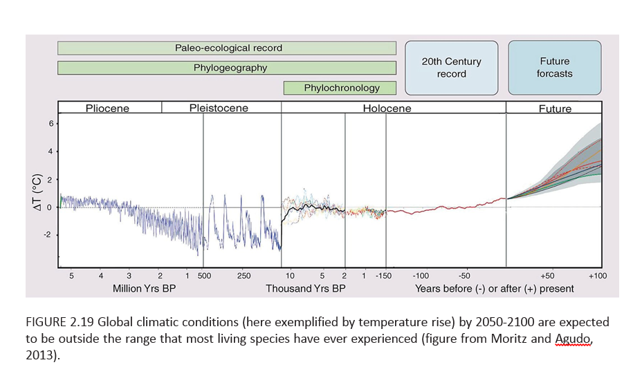
TempRise

So, for sure, there will be species extinction in the near term, hopefully not including the human species just yet.

Economic Impacts

In closing, I do think the primary obstacle to a sober evaluation of climate change involves social and economic implications. The climate change deniers may be right – acknowledging and adequately planning for responses to climate change would involve significant changes in social control and probably economic organization.

Of course, the AICH adopts a more moderate perspective – let’s be sure and set up monitoring of all this, so we can be prepared.

Hopefully, that will happen to some degree.

But adopting a more pro-active stance seems unlikely, at least in the near term. There is a wholesale rush to bringing one to several trillion persons who are basically living in huts with dirt floors into “the modern world.” Their children are traveling to cities, where they will earn much higher incomes, probably, and send money back home. The urge to have a family is almost universal, almost a concomitant of healthy love of a man and a woman. Tradeoffs between economic growth and environmental quality are a tough sell, when there are millions of new consumers and workers to be incorporated into the global supply chain. The developed nations – where energy and pollution output ratios are much better – are not persuasive when they suggest a developing giant like India or China should tow the line, limit energy consumption, throttle back economic growth in order to have a cooler future for the planet. You already got yours Jack, and now you want to cut back? What about mine? As standards of living degrade in the developed world with slower growth there, and as the wealthy grab more power in the situation, garnering even more relative wealth, the political dialogue gets stuck, when it comes to making changes for the good of all.

I could continue, and probably will sometime, but it seems to me that from a longer term forecasting perspective darker scenarios could well be considered. I’m sure we will see quite a few of these. One of the primary ones would be a kind of devolution of the global economy – the sort of thing one might expect if air travel were less possible because of, say, a major uptick in volcanism, or huge droughts took hold in parts of Asia.

Again and again, I come back to the personal thought of local self-reliance. There has been a growth with global supply chains and various centralizations, mergers, and so forth toward de-skilling populations, pushing them into meaningless service sector jobs (fast food), and losing old knowledge about, say, canning fruits and vegetables, or simply growing your own food. This sort of thing has always been a sort of quirky alternative to life in the fast lane. But inasmuch as life in the fast lane involves too much energy use for too many people to pursue, I think decentralized alternatives for lifestyle deserve a serious second look.

Polar bear on ice flow at top from http://metro.co.uk/2010/03/03/polar-bears-cling-to-iceberg-as-climate-change-ruins-their-day-141656/

Causal and Bayesian Networks

In his Nobel Acceptance Lecture, Sir C.J.W. Granger mentions that he did not realize people had so many conceptions of causality, nor that his proposed test would be so controversial – resulting in its being confined to a special category “Granger Causality.’

That’s an astute observation – people harbor many conceptions and shades of meaning for the idea of causality. It’s in this regard that renewed efforts recently – motivated by machine learning – to operationalize the idea of causality, linking it with both directed graphs and equation systems, is nothing less than heroic.

However, despite the confusion engendered by quantum theory and perhaps other “new science,” the identification of “cause” can be materially important in the real world. For example, if you are diagnosed with metastatic cancer, it is important for doctors to discover where in the body the cancer originated – in the lungs, in the breast, and so forth. This can be challenging, because cancer mutates, but making this identification can be crucial for selecting chemotherapy agents. In general, medicine is full of problems of identifying causal nexus, cause and effect.

In economics, Herbert Simon, also a Nobel Prize recipient, actively promoted causal analysis and its representation in graphs and equations. In Causal Ordering and Identifiability, Simon writes,

Simon1

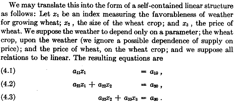
For example, we cannot reverse the causal chain poor growing weather → small wheat crops → increase in price of wheat by an attribution increase in price of wheat → poor growing weather.

Simon then proposes that the weather to price causal system might be represented by a series of linear, simultaneous equations, as follows:

Simon2

This example can be solved recursively, first by solving for x1, then by using this value of x1 to solve for x2, and then using the so-obtained values of x1 and x2 to solve for x3. So the system is self-contained, and Simon discusses other conditions. Probably the most important is assymmetry and the direct relationship between variables.

Readers interested in the milestones in this discourse, leading to the present, need to be aware of Pearl’s seminal 1998 article, which begins,

It is an embarrassing but inescapable fact that probability theory, the official mathematical language of many empirical sciences, does not permit us to express sentences such as “”Mud does not cause rain”; all we can say is that the two events are mutually correlated, or dependent – meaning that if we find one, we can expect to encounter the other.”

Positive Impacts of Machine Learning

So far as I can tell, the efforts of Simon and even perhaps Pearl would have been lost in endless and confusing controversy, were it not for the emergence of machine learning as a distinct specialization

A nice, more recent discussion of causality, graphs, and equations is Denver Dash’s A Note on the Correctness of the Causal Ordering Algorithm. Dash links equations with directed graphs, as in the following example.

DAGandEQS Dash shows that Simon’s causal ordering algorithm (COA) to match equations to a cluster graph is consistent with more recent methods of constructing directed causal graphs from the same equation set.

My reading suggests a direct line of development, involving attention to the vertices and nodes of directed acyclic graphs (DAG’s) – or graphs without any backward connections or loops – and evolution to Bayesian networks – which are directed graphs with associated probabilities.

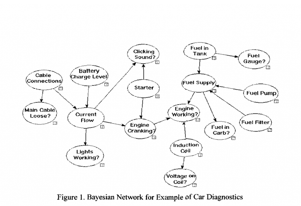
Here is are two examples of Bayesian networks.

First, another contribution from Dash and others

BayesNet

So clearly Bayesian networks are closely akin to expert systems, combining elements of causal reasoning, directed graphs, and conditional probabilities.

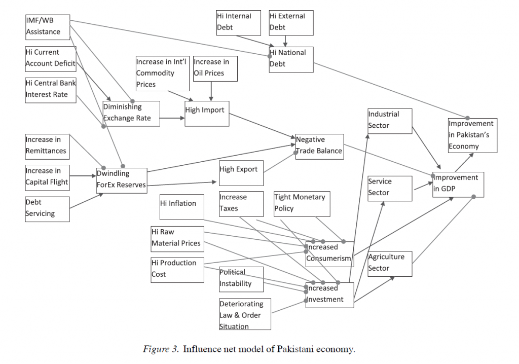
The scale of Bayesian networks can be much larger, or societal-wide, as this example from Using Influence Nets in Financial Informatics: A Case Study of Pakistan.

BnetPaki

The development of machine systems capable of responding to their environment – robots, for example – are a driver of this work currently. This leads to the distinction between identifying causal relations by observation or from existing data, and from intervention, action, or manipulation. Uncovering mechanisms by actively energizing nodes in a directed graph, one-by-one, is, in some sense, an ideal approach. However, there are clearly circumstances – again medical research provides excellent examples – where full-scale experimentation is simply not possible or allowable.

At some point, combinatorial analysis is almost always involved in developing accurate causal networks, and certainly in developing Bayesian networks. But this means that full implementation of these methods must stay confined to smaller systems, cut corners in various ways, or wait for development (one hopes) of quantum computers.

Note: header cartoon from http://xkcd.com/552/

Causal Discovery

So there’s a new kid on the block, really a former resident who moved back to the neighborhood with spiffy new toys – causal discovery.

Competitions and challenges give a flavor of this rapidly developing field – for example, the Causality Challenge #3: Cause-effect pairs, sponsored by a list of pre-eminent IT organizations and scientific societies (including Kaggle).

By way of illustration, B → A but A does not cause B – Why?

Kagglealttemp

These data, as the flipped answer indicates, are temperature and altitude of German cities. So altitude causes temperature, but temperature obviously does not cause altitude.

The non-linearity in the scatter diagram is a clue. Thus, values of variable A above about 130 map onto more than one value of B, which is problematic from conventional definition of causality. One cause should not have two completely different effects, unless there are confounding variables.

It’s a little fuzzy, but the associated challenge is very interesting, and data pairs still are available.

We provide hundreds of pairs of real variables with known causal relationships from domains as diverse as chemistry, climatology, ecology, economy, engineering, epidemiology, genomics, medicine, physics. and sociology. Those are intermixed with controls (pairs of independent variables and pairs of variables that are dependent but not causally related) and semi-artificial cause-effect pairs (real variables mixed in various ways to produce a given outcome).  This challenge is limited to pairs of variables deprived of their context.

Asymmetries As Clues to Causal Direction of Influence

The causal direction in the graph above is suggested by the non-invertibility of the functional relationship between B and A.

Another clue from reversing the direction of causal influence relates to the error distributions of the functional relationship between pairs of variables. This occurs when these error distributions are non-Gaussian, as Patrik Hoyer and others illustrate in Nonlinear causal discovery with additive noise models.

The authors present simulation and empirical examples.

Their first real-world example comes from data on eruptions of the Old Faithful geyser in Yellowstone National Park in the US.

OldFaithful Hoyer et al write,

The first dataset, the “Old Faithful” dataset [17] contains data about the duration of an eruption and the time interval between subsequent eruptions of the Old Faithful geyser in Yellowstone National Park, USA. Our method obtains a p-value of 0.5 for the (forward) model “current duration causes next interval length” and a p-value of 4.4 x 10⁻⁹ for the (backward) model “next interval length causes current duration”. Thus, we accept the model where the time interval between the current and the next eruption is a function of the duration of the current eruption, but reject the reverse model. This is in line with the chronological ordering of these events. Figure 3 illustrates the data, the forward and backward fit and the residuals for both fits. Note that for the forward model, the residuals seem to be independent of the duration, whereas for the backward model, the residuals are clearly dependent on the interval length.

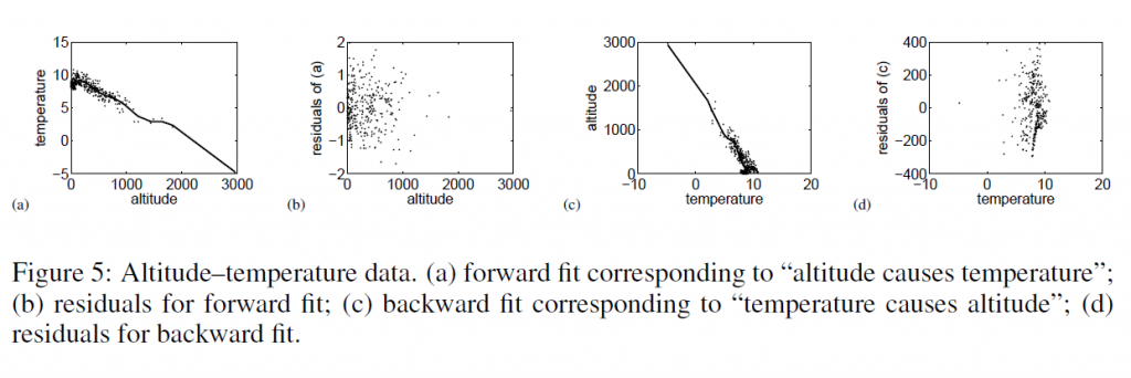
Then, they too consider temperature and altitude pairings.

tempaltHere, the correct model – altitude causes temperature – results in a much more random scatter of residuals, than the reverse direction model.

Patrik Hoyer and Aapo Hyvärinen are a couple of names from this Helsinki group of researchers whose papers are interesting to read and review.

One of the early champions of this resurgence of interest in causality works from a department of philosophy – Peter Spirtes. It’s almost as if the discussion of causal theory were relegated to philosophy, to be revitalized by machine learning and Big Data:

The rapid spread of interest in the last three decades in principled methods of search or estimation of causal relations has been driven in part by technological developments, especially the changing nature of modern data collection and storage techniques, and the increases in the processing power and storage capacities of computers. Statistics books from 30 years ago often presented examples with fewer than 10 variables, in domains where some background knowledge was plausible. In contrast, in new domains such as climate research (where satellite data now provide daily quantities of data unthinkable a few decades ago), fMRI brain imaging, and microarray measurements of gene expression, the number of variables can range into the tens of thousands, and there is often limited background knowledge to reduce the space of alternative causal hypotheses. Even when experimental interventions are possible, performing the many thousands of experiments that would be required to discover causal relationships between thousands or tens of thousands of variables is often not practical. In such domains, non-automated causal discovery techniques from sample data, or sample data together with a limited number of experiments, appears to be hopeless, while the availability of computers with increased processing power and storage capacity allow for the practical implementation of computationally intensive automated search algorithms over large search spaces.

Introduction to Causal Inference