Tag Archives: predictive analytics

cell phone data analytics, mobile ecommerce, technology forecasting

Mobile e-commerce

August 20, 2014 Clive Jones

Mobile ecommerce is no longer just another means consumers use to buy products online. It’s now the predominant way buyers visit ecommerce sites.

And mobile applications are radically changing the nature of shopping. The Emeritus founder of comScore, for example, highlights the two aspects of mobile ecommerce,

Examples of m-Shopping, according to Internet Retailer, include –

Online consumers use their smartphones and tablets for many shopping-related activities. In Q2 2013, 57% of smartphone users while in a retailer’s store visited that retailer’s site or app compared with 43% who consulted another company’s site or app, comScore says. The top reason consumers consulted retailers’ sites or apps was to compare prices. Among those smartphone users who went to the same retailer’s site, 59% wanted to see if there was an online discount available, the report says. Similarly, among those who checked a different retailer’s site, 92% wanted to see if they could get a better deal on price.

Smartphone owners also used their devices while in stores to take a picture of a product (23%), text or call family or friends about a product (17%), and send a picture of a product to family and friends (17%).

According to Gian Fulgoni, “m-Buying” is the predominant way shoppers now engage with retail brands online in the US.

Growth, Adoption, and Use of Mobile E-Commerce explores patterns of mobile ecommerce with extensive data on eBay transactions.

One of the more interesting findings is that,

..adoption of the mobile shopping application is associated with both an immediate and sustained increase in total platform purchasing. The data also do not suggest that mobile application purchases are simply purchases that would have been made otherwise on the regular Internet platform.

The following chart illustrates this effect.

Finally. responsive web design seems to be a key to optimizing for mobile ecommerce.

Responsive web design is a process of making your website content adaptable to the size of the screen you are viewing it on. By doing so, you can optimise your site for mobile and tablet traffic, without the need to manage multiple templates, or separate content.

A/B and Bandit Testing, Big Data, website optimization

E-Commerce Apps for Website Optimization

August 19, 2014 Clive Jones

There are dozens of web-based metrics for assessing ecommerce sites, but in the final analysis it probably just comes down to “conversion” rate. How many visitors to your ecommerce site end up buying your product or service?

Many factors come into play – such as pricing structure, product quality, customer service, and reputation.

But real-time predictive analytics plays an increasing role, according to How Predictive Analytics Is Transforming eCommerce & Conversion Rate Optimization. The author – Peep Laja – seems fond of Lattice, writing that,

Lattice has researched how leading companies like Amazon & Netflix are using predictive analytics to better understand customer behavior, in order to develop a solution that helps sales professionals better qualify their leads.

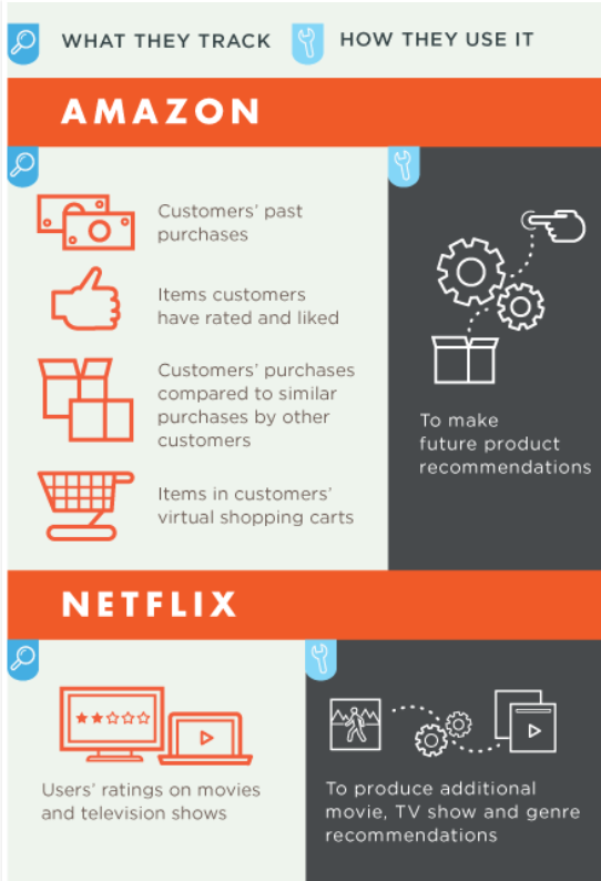
Laja also notes impressive success stories, such as Macy’s – which clocked an 8 to 12 percent increase in online sales by combining browsing behavior within product categories and sending targeted emails by customer segment.

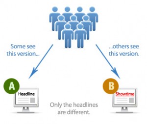
Google and Bandit Testing

I find the techniques associated with A/B or Bandit testing fascinating.

Google is at the forefront of this – the experimental testing of webpage design and construction.

Let me recommend readers directly to Google Analytics – the discussion headed by Overview of Content Experiments.

What is Bandit Testing?

Well, the Google presentation Multi-armed Bandits is really clear.

This is a fun topic.

So suppose you have a row of slot machine (“one-armed bandits”) and you know each machine has different probabilities and size of payouts. How do you decide which machine to favor, after a period of experimentation?

This is the multi-armed bandit or simply bandit problem, and is mathematically very difficult.

[The bandit problem] was formulated during the [second world] war, and efforts to solve it so sapped the energies and minds of Allied analysts that the suggestion was made that the problem be dropped over Germany, as the ultimate instrument of intellectual sabotage.

The Google discussion illustrates a Bayesian algorithm with simulations, showing that updating the probabilities and flow of traffic to what appear to be the most attractive web pages results, typically, in more rapid solutions that classical statistical experiments (generally known as A/B testing after “showroom A” and “showroom B”).

Suppose you’ve got a conversion rate of 4% on your site. You experiment with a new version of the site that actually generates conversions 5% of the time. You don’t know the true conversion rates of course, which is why you’re experimenting, but let’s suppose you’d like your experiment to be able to detect a 5% conversion rate as statistically significant with 95% probability. A standard power calculation1 tells you that you need 22,330 observations (11,165 in each arm) to have a 95% chance of detecting a .04 to .05 shift in conversion rates. Suppose you get 100 sessions per day to the experiment, so the experiment will take 223 days to complete. In a standard experiment you wait 223 days, run the hypothesis test, and get your answer.

Now let’s manage the 100 sessions each day through the multi-armed bandit. On the first day about 50 sessions are assigned to each arm, and we look at the results. We use Bayes’ theorem to compute the probability that the variation is better than the original2. One minus this number is the probability that the original is better. Let’s suppose the original got really lucky on the first day, and it appears to have a 70% chance of being superior. Then we assign it 70% of the traffic on the second day, and the variation gets 30%. At the end of the second day we accumulate all the traffic we’ve seen so far (over both days), and recompute the probability that each arm is best. That gives us the serving weights for day 3. We repeat this process until a set of stopping rules has been satisfied (we’ll say more about stopping rules below).

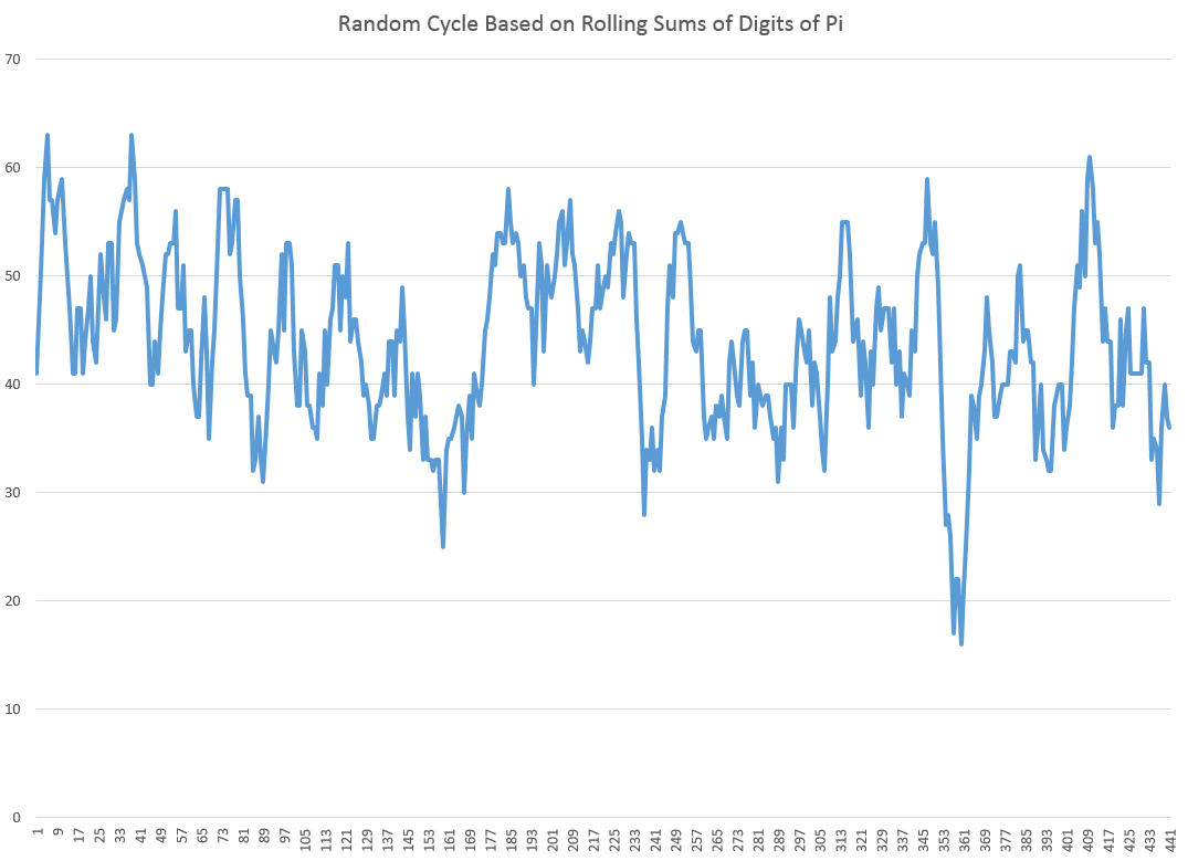
Figure 1 shows a simulation of what can happen with this setup. In it, you can see the serving weights for the original (the black line) and the variation (the red dotted line), essentially alternating back and forth until the variation eventually crosses the line of 95% confidence. (The two percentages must add to 100%, so when one goes up the other goes down). The experiment finished in 66 days, so it saved you 157 days of testing.

This Figure 1 chart is as follows.

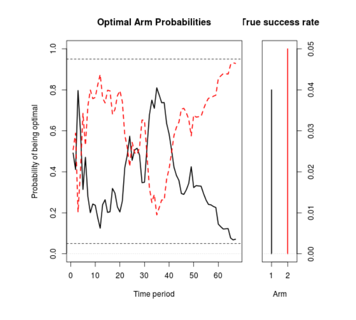
This is obviously just one outcome, but running this test many times verifies that in a majority of cases, the Google algorithm results in substantial shortening of test time, compared with an A/B test. In addition, if actual purchases are the meaning of “conversion” here, revenues are higher.

This naturally generalizes to any number of “arms” or slot machines.

Apparently, investors have put nearly $200 million in 2014 into companies developing predictive apps for ecommerce.

And, on the other side of the ledger, there are those who say that the mathematical training of people who might use these apps is still sub-par, and that the full potential of these techniques may not be realized in many cases.

The deeper analytics of the Google application is fascinating. It involves Monte Carlo simulation to integrate products of conditional and prior distributions, after new data comes in.

My math intuition, such as it is, suggests that this approach has wider applications. Why could it not, for example, be utilized for new products, where there might be two states, i.e. the product is a winner (following similar products in ramping up) or a loser? It’s also been used in speeding up health trials – an application of Bayesian techniques.

Top graphic from the One Hour Professor

IT market analysis, predictive analytics, technology forecasting

e-commerce and Forecasting

August 18, 2014 Clive Jones

The Census Bureau announced numbers from its latest e-commerce survey August 15.

The basic pattern continues. US retail e-commerce sales increased about 16 percent on a year-over-year basis from the second quarter of 2013. By comparison, total retail sales for the second quarter 2014 increased just short of 5 percent on a year-over-year basis.

As with other government statistics relating to IT (information technology), one can quarrel with the numbers (they may, for example, be low), but there is impressive growth no matter how you cut it.

Some of the top e-retailers from the standpoint of clicks and sales numbers are listed in Panagiotelis et al. Note these are sample data, from comScore with the totals for each company or site representing a small fraction of their actual 2007 online sales.

Forecasting Issues

Forecasting issues related to e-commerce run the gamut.

Website optimization and target marketing raise questions such as the profitability of “stickiness” to e-commerce retailers. There are advanced methods to tease out nonlinear, nonnormal multivariate relationships between, say, duration and page views and the decision to purchase – such as copulas previously applied in financial risk assessment and health studies.

Mobile e-commerce is a rapidly growing area with special platform and communications characteristics all its own.

Then, there are the pros and cons of expanding tax collection for online sales.

All in all, Darrell Rigby’s article in the Harvard Business Review – The Future of Shopping – is hard to beat. Traditional retailers generally have to move to a multi-channel model, supplementing brick-and-mortar stores with online services.

I plan several posts on these questions and issues, and am open for your questions.

Top graphic by DIGISECRETS

Big Data, gasoline price forecasts, geopolitical risk, predictive analytics

When the Going Gets Tough, the Tough Get Going

August 3, 2014 Clive Jones

Great phrase, but what does it mean? Well, maybe it has something to do with the fact that a lot of economic and political news seem to be entering kind of “end game.” But, it’s now the “lazy days of summer,” and there is a temptation to sit back and just watch it whiz by.

What are the options?

One is to go more analytical. I’ve recently updated my knowledge base on some esoteric topics –mathematically and analytically interesting – such as kernel ridge regression and dynamic principal components. I’ve previously mentioned these, and there are more instances of analysis to consider. What about them? Are they worth the enormous complexity and computational detail?

Another is to embrace the humming, buzzing confusion and consider “geopolitical risk.” The theme might be the price of oil and impacts, perhaps, of continuing and higher oil prices.

Or the proliferation of open warfare.

Rarely in recent decades have we seen outright armed conflict in Europe, as appears to be on-going in the Ukraine.

And I cannot make much sense of developments in the Mid-East, with some shadowy group called Isis scooping up vast amounts of battlefield armaments abandoned by collapsing Iraqi units.

Or how to understand Israeli bombardment of UN schools in Gaza, and continuing attacks on Israel with drones by Hamas. What is the extent and impact of increasing geopolitical risk?

There also is the issue of plague – most immediately ebola in Africa. A few days ago, I spent the better part of a day in the Boston Airport, and, to pass the time, read the latest Dan Brown book about a diabolical scheme to release an aerosol epidemic of sorts. In any case, ebola is in a way a token of a range of threats that stand just outside the likely. For example, there is the problem of the evolution of immune strains of bacteria, with widespread prescription and use.

There also is the ever-bloating financial bubble that has emerged in the US and elsewhere, as a result of various tactics of central and other banks in reaction to the Great Recession, and behavior of investors.

Finally, there are longer range scientific and technological possibilities. From my standpoint, we are making a hash of things generally. But efforts at political reform, by themselves, usually fall short, unless paralleled by fundamental new possibilities in production or human organization. And the promise of radical innovation for the betterment of things has never seemed brighter.

I will be exploring some of these topics and options in coming posts this week and in coming weeks.

And I think by now I have discovered a personal truth through writing – one that resonates with other experiences of mine professionally and personally. And that is sometimes it is just when the way to going further seems hard to make out that concentration of thought and energies may lead to new insight.

Big Data, business trends, IT market analysis, macroeconomic forecasting, technology forecasting

Links early August 2014

August 2, 2014 Clive Jones

Economy/Business

Economists React to July’s Jobs Report: ‘Not Weak, But…’

U.S. nonfarm employers added 209,000 jobs in July, slightly below forecasts and slower than earlier gains, while the unemployment rate ticked up to 6.2% from June. But employers have now added 200,000 or more jobs in six consecutive months for the first time since 1997.

The most important charts to see before the huge July jobs report – interesting to see what analysts were looking at just before the jobs announcement.

Despite sharp selloff, too early to worry about a correction

Venture Capital: Deals Beyond the Valley

7 Most Expensive Luxury Cars

Base price $136,000.

Contango And Backwardation Strategy For VIX ETFs Here you go!

Climate/Weather

Horrid California Drought Gets Worse Has a map showing drought conditions at intervals since 2011, dramatic.

Amazon’s Cloud Is Growing So Fast It’s Scaring Shareholders

Amazon has pulled off a pretty amazing trick over the past decade. It’s invented and then built a nearly $5 billion cloud computing business catering to fickle software developers and put the rest of the technology industry on the defensive. Big enterprise software companies such as IBM and HP and even Google are playing catchup, even as they acknowledge that cloud computing is the tech industry’s future.

But what kind of a future is that to be? Yesterday Amazon said that while its cloud business grew by 90 percent last year, it was significantly less profitable. Amazon’s AWS cloud business makes up the majority of a balance sheet item it labels as “other” (along with its credit card and advertising revenue) and that revenue from that line of business grew by 38 percent. Last quarter, revenue grew by 60 percent. In other words, Amazon is piling on customers faster than it’s adding dollars to its bottom line.

The Current Threat

Infographic: Ebola By the Numbers

Data Science

Statistical inference in massive data sets Interesting and applicable procedure illustrated with Internet traffic numbers.

business cycle, cycles, time series forecasting

Random Cycles

July 30, 2014 Clive Jones

In 1927, the Russian statistician Eugen Slutsky wrote a classic article called ‘The summation of random causes as the source of cyclic processes,’ a short summary of which is provided by Barnett –

If the variables that were taken to represent business cycles were moving averages of past determining quantities that were not serially correlated – either real-world moving averages or artificially generated moving averages – then the variables of interest would become serially correlated, and this process would produce a periodicity approaching that of sine waves

It’s possible to illustrate this phenomena with rolling sums of the digits of pi (π). The following chart illustrates the wave-like result of charting rolling sums of ten consecutive digits of pi.

So to be explicit, I downloaded the first 450 digits of pi, took them apart, and then graphed the first 440 rolling sums.

The wave-like pattern Illustrates a random cycle.

Forecasting Random Cycles

If we consider this as a time series, each element x_k is the following sum,

x_k = d_k+d_k-1+..+d_k-10

where dj is the jth digit in the decimal expansion of pi to the right of the initial value of 3.

Now, apparently, it is not proven that the digits of pi are truly random, although one can show that, so far as we can compute, these digits are described by a uniform distribution.

As far as we know, the probability that the next digit will be any digit from 0 to 9 is 1/10=0.1

So as one moves through the digits of pi, generating rolling sums, each new sum means the addition of a new digit, which is unknown and can only be predicted up to its probability. And, at the same time, a digit at the beginning of the preceding sum drops away in the new sum.

Note also that we can always deduce what the series of original digits is, given a series of these rolling sums up to some point.

So the issue is whether the new digit added to the next sum is greater than, equal to, or less than the leading digit of the current sum – which is where we now stand in this sort of analysis. This determines whether the next rolling sum will be greater than, equal to, or less than the current sum.

Here’s where the forecasts can be produced. If the rolling sum is large enough, approaching or equal to 90, there is a high probability that the next rolling sum will be lower, leading to this wave-like pattern. Conversely, if the rolling sum is near zero, the chances are the subsequent sum will be larger. And all this arm-waving can be complemented by exact probabilistic calculations.

Some Ultimate Thoughts

It’s interesting we are really dealing here with a random cycle. That’s proven by the fact that, at any time, the series could go flat-line or trace out some other kind of weird movement.

Thus, the quasi-periodic aspect can be violated for as many periods as you might choose, if one arrives at a run of the same digit in the expansion of pi.

This reminds me of something George Gamow wrote in one of his popular books, where he discusses thermodynamics and the random movement of atoms and molecules in the air of a room. Gamow observes it is entirely possible all the air by chance will congregate in one corner, leaving a vacuum elsewhere. Of course, this is highly improbable.

The only difference would be that there are a finite number of atoms and molecules in the air of any room, but, presumably, an infinite number of digits in the expansion of pi.

The morale of the story is, in any case, to be cautious in imposing a fixed cycle on this type of series.

accuracy of forecasts, analyzing seasonal effects, energy forecasting, gasoline price forecasts, long term forecasting, univariate forecast modeling approaches

Analyzing Complex Seasonal Patterns

July 15, 2014 Clive Jones

When time series data are available in frequencies higher than quarterly or monthly, many forecasting programs hit a wall in analyzing seasonal effects.

Researchers from the Australian Monash University published an interesting paper in the Journal of the American Statistical Association (JASA), along with an R program, to handle this situation – what can be called “complex seasonality.”

I’ve updated and modified one of their computations – using weekly, instead of daily, data on US conventional gasoline prices – and find the whole thing pretty intriguing.

If you look at the color codes in the legend below the chart, it’s a little easier to read and understand.

Here’s what I did.

I grabbed the conventional weekly US gasoline prices from FRED. These prices are for “regular” – the plain vanilla choice at the pump. I established a start date of the first week in 2000, after looking the earlier data over. Then, I used tbats(.) in the Hyndman R Forecast package which readers familiar with this site know can be downloaded for use in the open source matrix programming language R.

Then, I established an end date for a time series I call newGP of the first week in 2012, forecasting ahead with the results of applying tbats(.) to the historic data from 2000:1 to 2012:1 where the second number refers to weeks which run from 1 to 52. Note that some data scrubbing is needed to shoehorn the gas price data into 52 weeks on a consistent basis. I averaged “week 53” with the nearest acceptable week (either 52 or 1 in the next year), and then got rid of the week 53’s.

The forecast for 104 weeks is shown by the solid red line in the chart above.

This actually looks promising, as if it might encode some useful information for, say, US transportation agencies.

A draft of the JASA paper is available as a PDF download. It’s called Forecasting time series with complex seasonal patterns using exponential smoothing and in addition to daily US gas prices, analyzes daily electricity demand in Turkey and bank call center data.

I’m only going part of the way to analyzing the gas price data, since I have not taken on daily data yet. But the seasonal pattern identified by tbats(.) from the weekly data is interesting and is shown below.

The weekly frequency may enable us to “get inside” a mid-year wobble in the pattern with some precision. Judging from the out-of-sample performance of the model, this “wobble” can in some cases be accentuated and be quite significant.

Trignometric series fit to the higher frequency data extract the seasonal patterns in tbats(.), which also features other advanced features, such as a capability for estimating ARMA (autoregressive moving average) models for the residuals.

I’m not fully optimizing the estimation, but these results are sufficiently strong to encourage exploring the toggles and switches on the routine.

Another routine which works at this level of aggregation is the stlf(.) routine. This is uses STL decomposition described in some detail in Chapter 36 Patterns Discovery Based on Time-Series Decomposition in a collection of essays on data mining.

Thoughts

Good forecasting software elicits sort of addictive behavior, when initial applications of routines seem promising. How much better can the out-of-sample forecasts be made with optimization of the features of the routine? How well does the routine do when you look at several past periods? There is even the possibility of extracting further information from the residuals through bootstrapping or bagging at some point. I think there is no other way than exhaustive exploration.

The payoff to the forecaster is the amazement of his or her managers, when features of a forecast turn out to be spot-on, prescient, or what have you – and this does happen with good software. An alternative, for example, to the Hyndman R Forecast package is the program STAMP I also am exploring. STAMP has been around for many years with a version running – get this – on DOS, which appears to have had more features than the current Windows incarnation. In any case, I remember getting a “gee whiz” reaction from the executive of a regional bus district once, relating to ridership forecasts. So it’s fun to wring every possible pattern from the data.

accuracy of forecasts, global business forecasts

Seasonal Sales Patterns – Stylized Facts

July 14, 2014 Clive Jones

Seasonal sales patterns in the United States are more or less synchronized with Europe, Japan, China, and, to a lesser extent, the rest of the world.

Here are some stylized facts:

Sales tend to peak at the end of the calendar year. This is the well-known “Christmas effect,” and is a strong enough factor to “cannibalize” demand, to an extent, at the first of the following year.
Sales of final goods tend to be lower – in terms of growth rates and, in some cases, absolutely, in the first calendar quarter of the year.
Supply chain effects, related to pulses of sales of final goods, can be identified for various lines of production depending on production lead times. Semiconductor orders, for example, tend to peak earlier than sales of consumer electronics, which are sharply influenced by the Christmas season.

To validate this picture, let me offer some evidence.

First, consider retail and food service sales data for the US, a benchmark of consumer activity – the recently discussed data downloaded from FRED.

Applying the automatic model selection of the Hyndman R Forecast package, we get a decomposition of this time series into level, trend, and seasonals, as shown in the following diagram.

The optimal exponential smoothing forecast model is a model with a damped trend and multiplicative seasonals.

If we look at the lower part of this diagram, we see that the seasonal factor for December – which is shown by the major peaks in the curve – is a multiple of more than 1.15. On the other hand, the immediately following month – January – shows a multiple of 0.9. These factors are multiplied into the product of the level and trend to get the sales for December and January. In other words, you can suppose that, roughly speaking, December retail sales will be 15 percent above trend, while January sales will be 90 percent of trend.

And, if you inspect this diagram in the lower panel carefully, you can detect the lull in late summer and fall in retail sales.

With “just-in-time” inventories and lean production models, actual production activity closely tracks these patterns in final demand – although it does take some lead time to produce stuff.

These stylized facts have not changed in their outlines since the ground-breaking research of Jeffrey Miron in the the late 1980’s. Miron refers to a worldwide seasonal cycle in aggregate economic activity whose major features are a fourth quarter boom in output.., a third quarter trough in manufacturing production, and a first quarter trough in all economic activity.

The Effects of Different Calendars – the Chinese New Year and Ramadan

The Gregorian calendar has achieved worldwide authority, and almost every country follows on the conventions of counting the year (currently 2014).

The Chinese calendar, however, is still important for determining the timing of festivals for Chinese communities around the world, and, especially, in China.

Similarly, the Islamic calendar governs the timing of important ritual periods and religious festivals – such as the month of Ramadan, which falls in June and July in 2014.

Because these festival periods overlap with multiple Gregorian months, there can be significant localized impacts on estimates of seasonal variation of economic activity.

Taiwanese researchers looking at this issue find significant holiday effects, related the fact that,

The three most important Chinese holidays, Chinese New Year, the Dragon-boat Festival, and Mid-Autumn Holiday have dates determined by a lunar calendar and move between two solar months. Consumption, production, and other economic behavior in countries with large Chinese population including Taiwan are strongly affected by these holidays. For example, production accelerates before lunar new year, almost completely stops during the holidays and gradually rises to an average level after the holidays.

accuracy of forecasts, financial forecasting, IT market analysis, predictive analytics, stock market forecasts

The NASDAQ 100 Daily Returns and Laplace Distributed Errors

June 24, 2014 Clive Jones

I once ran into Norman Mailer at the Museum of Modern Art in Manhattan. We were both looking at Picasso’s “Blue Boy” and, recognizing him, I started up some kind of conversation, and Mailer was quite civil about the whole thing.

I mention this because I always associate Mailer with his collection Advertisements for Myself.

And that segues – loosely – into my wish to let you know that, in fact, I developed a generalization of the law of demand for the situation in which a commodity is sold at a schedule of rates and fees, instead of a uniform price. That was in 1987, when I was still a struggling academic and beginning a career in business consulting.

OK, and that relates to a point I want to suggest here. And that is that minor players can have big ideas.

So I recognize an element of “hubris” in suggesting that the error process of S&P 500 daily returns – up to certain transformations – is described by a Laplace distribution.

What about other stock market indexes, then? This morning, I woke up and wondered whether the same thing is true for, say, the NASDAQ 100.

So I downloaded daily closing prices for the NASDAQ 100 from Yahoo Finance dating back to October 1, 1985. Then, I took the natural log of each of these closing prices. After that, I took trading day by trading day differences. So the series I am analyzing comes from the first differences of the natural log of the NASDAQ 100 daily closing prices.

Note that this series of first differences is sometimes cast into a histogram by itself – and this also frequently is a “pointy peaked” relatively symmetric distribution. You could motivate this graph with the idea that stock prices are a random walk. So if you take first differences, you get the random component that generates the random walk.

I am troubled, however, by the fact that this component has considerable structure in and of itself. So I undertake further analysis.

For example, the autocorrelation function of these first differences of the log of NASDAQ 100 daily closing prices looks like this.

Now if you calculate bivariate regressions on these first differences and their lagged values, many of them produce coefficient estimates with t-statistics that exceed the magic value of 2.

Just selecting these significant regressors from the first 47 lags produces this regression equation, I get this equation.

Now this regression is estimated over all 7200 observations from October 1 1984 to almost right now.

Graphing the residuals, I get the familiar pointy-peaked distribution that we saw with the S&P 500.

Here is a fit of the Laplace distribution to this curve (Again using EasyFit).

Here are the metrics for this fit and fits to a number of other probability distributions from this program.

I have never seen as clear a linkage of returns from stock indexes and the Laplace distribution (maybe with a slight asymmetry – there are also asymmetric Laplace distributions).

One thing is for sure – the distribution above for the NASDAQ 100 data and the earlier distribution developed for the S&P 500 are not close to be normally distributed. Thus, in the table above that the normal distribution is number 12 on the list of possible candidates identified by EasyFit.

Note “Error” listed in the above table, is not the error function related to the normal distribution. Instead it is another exponential distribution with an absolute value in the exponent like the Laplace distribution. In fact, it looks like a transformation of the Laplace, but I need to do further investigation. In any case, it’s listed as number 2, even though the metrics show the same numbers.

The plot thickens.

Obviously, the next step is to investigate individual stocks with respect to Laplacian errors in this type of transformation.

Also, some people will be interested in whether the autoregressive relationship listed above makes money under the right trading rules. I will report further on that.

Anyway, thanks for your attention. If you have gotten this far – you believe numbers have power. Or you maybe are interested in finance and realize that indirect approaches may be the best shot at getting to something fundamental.

accuracy of forecasts, analytical software, financial forecasting, probability distribution analysis, stock market forecasts

The Laplace Distribution and Financial Returns

June 23, 2014 Clive Jones

Well, using EasyFit from Mathwave, I fit a Laplace distribution to the residuals of the regression on S&P daily returns I discussed yesterday.

Here is the result.

This beats a normal distribution hands down. It also appears to beat the Matlab fit of a t distribution, but I have to run down more details on forms of the t-distribution to completely understand what is going on in the Matlab setup.

Note that EasyFit is available for a free 30-day trial download. It’s easy to use and provides metrics on goodness of fit to make comparisons between distributions.

There is a remarkable book online called The Laplace Distribution and Generalizations. If you have trouble downloading it from the site linked here, Google the title and find the download for a free PDF file.

This book, dating from 2001, runs to 458 pages, has a good introductory discussion, extensive mathematical explorations, as well as applications to engineering, physical science, and finance.

The French mathematical genius Pierre Simon Laplace proposed the distribution named after him as a first law of errors when he was 25, before his later discussions of the normal distribution.

The normal probability distribution, of course, “took over” – in part because of its convenient mathematical properties and also, probably, because a lot of ordinary phenomena are linked with Gaussian processes.

John Maynard Keynes, the English economist, wrote an early monograph (Keynes, J.M. (1911). The principal averages and the laws of error which lead to them, J. Roy. Statist. Soc. 74, New Series, 322-331) which substantially focuses on the Laplace distribution, highlighting the importance it gives to the median, rather than average, of sample errors.

The question I’ve struggled with is “why should stock market trading, stock prices, stock indexes lead, after logarithmic transformation and first differencing to the Laplace distribution?”

Of course, the Laplace distribution can be generated as a difference of exponential distributions, or as combination of a number of distributions, as the following table from Kotz, Kozubowski, and Podgorski’s book shows.

This is all very suggestive, but how can it be related to the process of trading?

Indeed, there are quite a number of questions which follow from this hypothesis – that daily trading activity is fundamentally related to a random component following a Laplace distribution.

What about regression, if the error process is not normally distributed? By following the standard rules on “statistical significance,” might we be led to disregard variables which are drivers for daily returns or accept bogus variables in predictive relationships?

Distributional issues are important, but too frequently disregarded.

I recall a blog discussion by a hedge fund trader lamenting excesses in the application of the Black-Scholes Theorem to options in 2007 and thereafter.

Possibly, the problem is as follows. The residuals of autoregressions on daily returns and their various related transformations tend to cluster right around zero, but have big outliers. This clustering creates false confidence, making traders vulnerable to swings or outliers that occur much more frequently than suggested by a normal or Gaussian error distribution.

Business Forecasting